The ad.linalg submodule was created to overcome the limitations of performing AD with compiled numerical routines (e.g., LAPACK). The following algorithms have a translation that are AD-compatible:
Each item listed above is a NumPy-equivalent function, though not completely interchangeable. The descriptions that follow are not meant to introduce theory for the methods, nor to show an exhaustive set of examples as to their usage. They simply describe the respective algorithm’s usage with some relevant examples. Several algorithms have been borrowed from the tasks described at RosettaCode.
Cholesky decomposition involves taking a symmetric, positive-definite matrix A and decomposing it into L such that A=LL’=U’U, where L is a lower triangular matrix and U is an upper triangular matrix.
Example 1:
>>> A = [[25, 15, -5],
...      [15, 18,  0],
...      [-5,  0, 11]]
...
>>> L = chol(A)
>>> L
array([[ 5.,  0.,  0.],
       [ 3.,  3.,  0.],
       [-1.,  1.,  3.]])
>>> U = chol(A, 'upper')
>>> U
array([[ 5.,  3., -1.],
       [ 0.,  3.,  1.],
       [ 0.,  0.,  3.]])
Example 2:
>>> A = [[18, 22,  54,  42],
...      [22, 70,  86,  62],
...      [54, 86, 174, 134],
...      [42, 62, 134, 106]]
...
>>> L = chol(A)
>>> L
array([[  4.24264069,   0.        ,   0.        ,   0.        ],
       [  5.18544973,   6.5659052 ,   0.        ,   0.        ],
       [ 12.72792206,   3.0460385 ,   1.64974225,   0.        ],
       [  9.89949494,   1.62455386,   1.84971101,   1.39262125]])
LU Decomposition factors a matrix as the product of a lower triangular matrix and an upper triangular matrix, and in this case, a pivot or permutation matrix as well. The decomposition can be viewed as the matrix form of gaussian elimination. Computers usually solve square systems of linear equations using the LU decomposition, and it is also a key step when inverting a matrix, or computing the determinant of a matrix.
Example 1:
>>> A = [[1, 3, 5],
...      [2, 4, 7],
...      [1, 1, 0]]
...
>>> L, U, P = lu(A)
>>> L
array([[ 1. ,  0. ,  0. ],
       [ 0.5,  1. ,  0. ],
       [ 0.5, -1. ,  1. ]])
>>> U
array([[ 2. ,  4. ,  7. ],
       [ 0. ,  1. ,  1.5],
       [ 0. ,  0. , -2. ]])
>>> P
array([[ 0.,  1.,  0.],
       [ 1.,  0.,  0.],
       [ 0.,  0.,  1.]])
Example 2:
>>> A = [[11,  9, 24, 2],
...      [ 1,  5,  2, 6],
...      [ 3, 17, 18, 1],
...      [ 2,  5,  7, 1]]
...
>>> L, U, P = lu(A)
>>> L
array([[ 1.        ,  0.        ,  0.        ,  0.        ],
       [ 0.27272727,  1.        ,  0.        ,  0.        ],
       [ 0.09090909,  0.2875    ,  1.        ,  0.        ],
       [ 0.18181818,  0.23125   ,  0.00359712,  1.        ]])
>>> U
array([[ 11.        ,   9.        ,  24.        ,   2.        ],
       [  0.        ,  14.54545455,  11.45454545,   0.45454545],
       [  0.        ,   0.        ,  -3.475     ,   5.6875    ],
       [  0.        ,   0.        ,   0.        ,   0.51079137]])
>>> P
array([[ 1.,  0.,  0.,  0.],
       [ 0.,  0.,  1.,  0.],
       [ 0.,  1.,  0.,  0.],
       [ 0.,  0.,  0.,  1.]])
QR decomposition is applicable to any m-by-n matrix A and decomposes into A=QR where Q is an orthogonal matrix of size m-by-m and R is an upper triangular matrix of size m-by-n. QR decomposition provides an alternative way of solving the systems of equations Ax=b without inverting the matrix A. The fact that Q is orthogonal means that Q’Q=I, so that Ax=b is equivalent to Rx=Q’b, which is easier to solve since R is triangular.
Example of a square input matrix:
>>> A = [[12, -51,   4],
...      [ 6, 167, -68],
...      [-4,  24, -41]]
...
>>> q, r = qr(A)
>>> q
array([[-0.85714286,  0.39428571,  0.33142857],
       [-0.42857143, -0.90285714, -0.03428571],
       [ 0.28571429, -0.17142857,  0.94285714]])
>>> r
array([[ -1.40000000e+01,  -2.10000000e+01,   1.40000000e+01],
       [  5.97812398e-18,  -1.75000000e+02,   7.00000000e+01],
       [  4.47505281e-16,   0.00000000e+00,  -3.50000000e+01]])
Example of a non-square input matrix:
>>> A = [[12, -51,   4],
...      [ 6, 167, -68],
...      [-4,  24, -41],
...      [-1,   1,   0],
...      [ 2,   0,   3]]
...
>>> q, r = qr(A)
>>> q
array([[-0.84641474,  0.39129081, -0.34312406,  0.06613742, -0.09146206],
       [-0.42320737, -0.90408727,  0.02927016,  0.01737854, -0.04861045],
       [ 0.28213825, -0.17042055, -0.93285599, -0.02194202,  0.14371187],
       [ 0.07053456, -0.01404065,  0.00109937,  0.99740066,  0.00429488],
       [-0.14106912,  0.01665551,  0.10577161,  0.00585613,  0.98417487]])
>>> r
array([[ -1.41774469e+01,  -2.06666265e+01,   1.34015667e+01],
       [  3.31666807e-16,  -1.75042539e+02,   7.00803066e+01],
       [ -3.36067949e-16,   2.87087579e-15,   3.52015430e+01],
       [  9.46898347e-17,   5.05117109e-17,  -9.49761103e-17],
       [ -1.74918720e-16,  -3.80190411e-16,   8.88178420e-16]])
>>> import numpy as np
>>> np.all(np.dot(q, r) - A<1e-12)
True
The general solver for linear systems of equations uses gaussian elimination. One or multiple columns in the RHS can be input, like when solving for the matrix inverse.
Example:
>>> A = [[1, 2, 1], [4, 6, 3], [9, 8, 2]]
>>> b = [3, 2, 1]
>>> solve(A, b)
array([ -7.,  11., -12.])
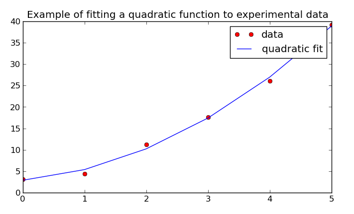
Solving a system of linear equations using the least squares method involves the usage of QR decomposition.
Example: Fit a quadratic line to some experimental data:
>>> x = np.array([0, 1, 2, 3, 4, 5])
>>> y = np.array([3, 6, 11, 18, 27, 38])
>>> y = y + np.random.randn(len(y))  # give the output a random offset
>>> A = np.vstack([np.ones(len(x)), x, x**2]).T
>>> A
array([[  1.,   0.,   0.],
       [  1.,   1.,   1.],
       [  1.,   2.,   4.],
       [  1.,   3.,   9.],
       [  1.,   4.,  16.],
       [  1.,   5.,  25.]])
>>> b = lstsq(A, y)  # the quadratic fit coefficients (b0 + b1*x + b2*x**2)
Now, we can see what the fit looks like compared to the original data using Matplotlib:
>>> fit = lambda x: b[0] + b[1]*x + b[2]*x**2
>>> import matplotlib.pyplot as plt
>>> plt.plot(x, y, 'ro', x, fit(x), 'b-')
>>> plt.legend(['data', 'quadratic fit'])
>>> plt.show()
Solving for a matrix inverse is performed using inv(). Internally, this is done using the general solver and inputting the an appropriately sized identity matrix as the RHS of the system.
Example:
>>> A = [[25, 15, -5],
...      [15, 18,  0],
...      [-5,  0, 11]]
...
>>> Ainv = inv(A)
>>> Ainv
array([[ 0.09777778, -0.08148148,  0.04444444],
       [-0.08148148,  0.12345679, -0.03703704],
       [ 0.04444444, -0.03703704,  0.11111111]])
>>> np.dot(Ainv, A)
array([[  1.00000000e+00,   0.00000000e+00,   0.00000000e+00],
       [  2.77555756e-16,   1.00000000e+00,   0.00000000e+00],
       [  0.00000000e+00,   1.11022302e-16,   1.00000000e+00]])
You’ll notice that the off-diagonal elements aren’t all perfectly zero. This is due to floating-point error, but otherwise the final matrix is the identity matrix.
