Tensor Wrapper

The tensor wrapper is a data structure which mimics the behavior of a numpy.ndarray and associates each item of the tensor with the evaluation of a user-defined function on the corresponding grid point.

Let for example \(\mathcal{X} = \times_{i=1}^d {\bf x}_i\), where \({\bf x}_i\) define the position of the grid points in the \(i\)-th direction. Let us consider the function \(f:\mathcal{X}\rightarrow \mathbb{R}^{n_1\times \ldots \times n_m}\). Let us define the tensor valued tensor \(\mathcal{A}=f(\mathcal{X})\). Thus any entry \(\mathcal{A}[i_1,\ldots,i_d] = f({\bf x}_{i_1},\ldots,{\bf x}_{i_d})\) is a tensor in \(\mathbb{R}^{n_1\times \ldots \times n_m}\). The storage of the whole tensor \(\mathcal{A}\) can be problematic for big \(d\) and \(m\), and not necessary if one is just willing to sample values from it.

The TensorWrapper allows the access to the elements of \(\mathcal{A}\) which however are not all allocated, but computed on-the-fly and stored in a hash-table data structure (a Python dictionary). The TensorWrapper can be reshaped and accessed as if it was a numpy.ndarray (including slicing of indices). Additionally it allows the existence of multiple views of the tensor, sharing among them the allocated data, and it allows the Quantics folding used within the Quantics Tensor Train [2][1] routines QTTvec.

In the following we will use a simple example to show the capabilities of this data structure. We will let \(d=2\) and \(f:\mathcal{X}\rightarrow \mathbb{R}\).

Construction

In order to construct a TensorWrapper we need first to define a grid and a function.

>>> import numpy as np
>>> import itertools
>>> import TensorToolbox as TT
>>> d = 2
>>> x_fine = np.linspace(-1,1,7)
>>> params = {'k': 1.}
>>> def f(X,params):
>>>     return np.max(X) * params['k']
>>> TW = TT.TensorWrapper( f, [ x_fine ]*d, params, dtype=float )

Access and data

The TensorWrapper can then be accessed as a numpy.ndarray:

>>> TW[1,2]
-0.33333333333333337

This access to the TensorWrapper has caused the evaluation of the function \(f\) and the storage of the associated value. In order to check the fill level of the TensorWrapper, we do:

>>> TW.get_fill_level()
1

The evaluation indices at which the function has been evaluated can be retrived this way:

>>> TW.get_fill_idxs()
[(1, 2)]

The TensorWrapper can be accessed using also slicing along some of the coordinates:

>>> TW[:,1:6:2]
array([[-0.66666666666666674, 0.0, 0.66666666666666652],
    [-0.66666666666666674, 0.0, 0.66666666666666652],
    [-0.33333333333333337, 0.0, 0.66666666666666652],
    [0.0, 0.0, 0.66666666666666652],
    [0.33333333333333326, 0.33333333333333326, 0.66666666666666652],
    [0.66666666666666652, 0.66666666666666652, 0.66666666666666652],
    [1.0, 1.0, 1.0]], dtype=object)

The data already computed are stored in the dictionary TensorWrapper.data, which one can access and modify at his/her own risk. The data can be erased just by resetting the TensorWrapper.data field:

>>> TW.data = {}

The constructed TensorWrapper to which has not been applied any of the view/extension/reshaping functions presented in the following, is called the global tensor wrapper. The shape informations regarding the global wrapper can be always accessed by:

>>> TW.get_global_shape()
(7, 7)
>>> TW.get_global_ndim()
2
>>> TW.get_global_size()
49

If no view/extension/reshaping has been applied to the TensorWrapper, then the same output is obtained by:

>>> TW.get_shape()
(7, 7)
>>> TW.get_ndim()
2
>>> TW.get_size()
49

or by

>>> TW.shape
(7, 7)
>>> TW.ndim
2
>>> TW.size
49

Note

If any view/extension/reshape has been applied to the TensorWrapper, then the output of TensorWrapper.get_global_shape() and TensorWrapper.get_shape() will differ. Anyway TensorWrapper.get_global_shape() will always return the information regarding the global tensor wrapper.

Views

The TensorWrapper allows the definition of multiple views over the defined tensor. The information regarding each view are contained in the dictionary TensoWrapper.maps. The main view is called full and is defined at construction time. Additional views can be defined through the function TensorWrapper.set_view(). Let’s continue the previous example, by adding a new view to the wrapper with a coarser grid.

>>> x_coarse = np.linspace(-1,1,4)
>>> TW.set_view( 'coarse', [x_coarse]*d )

Note

The grid of the full view must contain the grids associated to the new view.

The different views can be accessed separately, but they all refer to the same global data structure. In order to access the TensorWrapper through one of its views, the view must be activated:

>>> TW.set_active_view('coarse')
>>> TW[2,:]
>>> TW.set_active_view('full')
>>> TW[1,:]
>>> TW[:,2]

The following figure shows the global grid as well as its two views, the full and the coarse views. The allocated indicies are also highlighted.

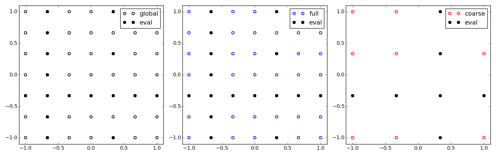
The global tensor and two of its views. The full view corresponds by default to the global tensor. The coarse is contained in the full view. The uniquely allocated values of the tensor are shown in the different views.

The shape characteristics of the active view can be accessed through TensorWrapper.get_view_shape() and the corresponding commands for ndim and size. For example:

>>> TW.set_active_view('full')
>>> TW.get_view_shape()
(7, 7)
>>> TW.get_shape()
(7, 7)
>>> TW.set_active_view('coarse')
>>> TW.get_global_shape()
(7, 7)
>>> TW.get_view_shape()
(4, 4)
>>> TW.get_shape()
(4, 4)
>>> TW.shape
(4, 4)

Grid refinement

The global grid can be refined using the function TensorWrapper.refine(), provinding a grid which contains the previous one. This refinement does not alter the allocated data which is instead preserved and mapped to the new mesh.

>>> x_ffine = np.linspace(-1,1,13)
>>> TW.refine([x_ffine]*d)

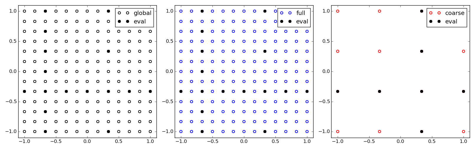
The global tensor and the two views defined, after the grid refinement.

Quantics extension

The quantics extension is used for extending the indices of the tesnor to the next power of Q. The extension is performed so that the last coordinate point is appended to the coordinate points the necessary number of times. In order to apply the extension on a particular view, one needs to activate the view and then use the method TensorWrapper.set_Q().

>>> TW.set_active_view('full')
>>> TW.get_view_shape()
(13, 13)
>>> TW.get_extended_shape()
(13, 13)
>>> TW.set_Q(2)
>>> TW.get_extended_shape()
(16, 16)
>>> TW.get_shape()
(16, 16)
>>> TW.shape
(16, 16)

We can see that TensorWrapper.get_extended_shape() returns the same output of TensorWrapper.get_viw_shape() if no quantics extension has been applied.

Using the following code we can investigate the content of the extended tensor wrapper and plot it as shown in the following figure.

>>> A = TW[:,:]
>>> import matplotlib.pyplot as plt
>>> plt.figure(figsize=(6,5))
>>> plt.imshow(A,interpolation='none')
>>> plt.tight_layout()
>>> plt.show(False)

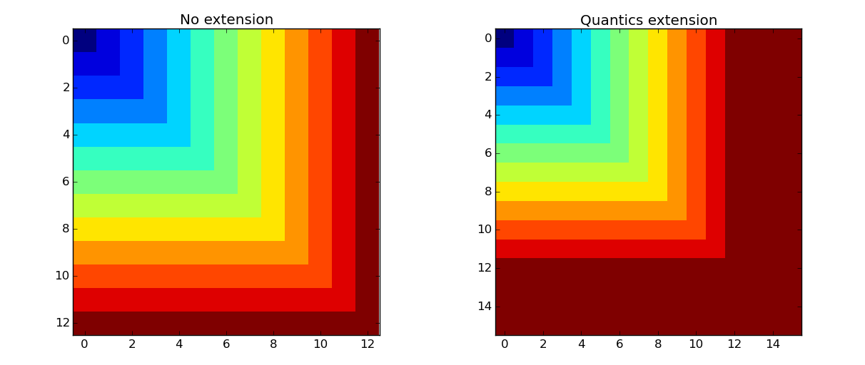
The Quantics extension applied to the full view results in the repetition of its limit values in the tensor grid.

Reshape

The shape of each view can be changed as long as the size returned by TensorWrapper.get_extended_size() is unchanged. This means that if no quantics extension has been applied, the size must correspond to TensorWrapper.get_view_size(). If a quantics extension has been applied, the size must correspond to TensorWrapper.get_extended_size().

For example let us reshape the quantics extended full view of the tensor to the shape (4,16).

>>> TW.set_active_view('full')
>>> TW.reshape((8,32))
>>> TW.get_extended_shape()
(16, 16)
>>> TW.get_shape()
(8, 32)
>>> TW.shape
(8, 32)

This results in the following reshaping of the tensor view:

>>> A = TW[:,:]
>>> import matplotlib.pyplot as plt
>>> plt.figure(figsize=(12,5))
>>> plt.imshow(A,interpolation='none')
>>> plt.tight_layout()
>>> plt.show(False)

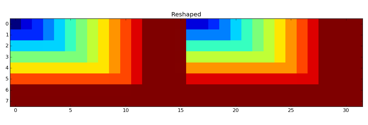
Reshaping of the quantics extended full view.

The quantics extension is used mainly to obtain a complete folding of base Q. In this case this is obtained by:

>>> import math
>>> TW.reshape( [2] * int(round(math.log(TW.size,2))) )
>>> TW.get_extended_shape()
(16, 16)
>>> TW.get_shape()
(2, 2, 2, 2, 2, 2, 2, 2)
>>> TW.shape
(2, 2, 2, 2, 2, 2, 2, 2)

We finally can reset the shape to the view shape using:

>>> TW.reset_shape()

Summary of shapes

Information regarding several shape transformations are always hold in the data structure. A hierarchy of shapes is used. The top shape is the global shape. In the following table we list the different shapes, their description and the main functions related and affecting them.

Shape	Description	Functions
Global	This is the underlying shape of the TensorWrapper.	get_global_shape(), get_global_ndim(), get_global_size(), refine()
View	Multiple views can be defined for a TensorWrapper. The views are defined as nested grids into the global grid. The default view is called full and is defined automatically at construction time	set_view(), set_active_view(), get_view_shape(), get_view_ndim(), get_view_size(), refine()
Quantics Extended	Each view can be extended to the next power of Q in order to allow the quantics folding [2][1] of the tensor.	set_Q(), get_extended_shape(), get_extended_ndim(), get_extended_size()
Reshape	This is the result of the reshape of the tensor. If any of the preceding shape transformations have been applied, then the reshape is applied to the lowest transformation.	reshape(), get_shape(), get_ndim(), get_size(), shape, ndim, size

Warning

If a shape at any level is modified, every lower reshaping is automatically erased, due to possible inconsistency. For example, if a view is modified, any quantics extension and/or reshape of the view are reset.

Note

The refine() function erases all the quantics extensions and the reshapes of each view, but not the views themselves. Instead for each view, the refine() function updates the corresponding indices, fitting the old views to the new refinement.

Storage

Instances of the class TensorWrapper can be stored in files and reloaded as needed. The class TensorWrapper extends the class storable_object, which is responsible for storing objects in the TensorToolbox.

For the sake of efficiency and readability of the code, the TensorWrapper is stored in two different files with a common file name filename:

• filename.pkl is a serialized version of the object thorugh the pickle library. The TensorWrapper serializes a minimal amount of auxiliary information needed for the definition of shapes, meshes, etc. The allocated data are not serialized using pickle, because when the amount of data is big, this would result in a very slow storage.
• filename.h5 is a binary file containing the allocated data of the TensorWrapper. This file is generated using h5py and results in fast loading, writing and appending of data.

Let us store the TensorWrapper, we have been using up to now.

>>> TW.set_store_location('tensorwrapper')
>>> TW.store(force=True)

Check that the files have been stored:

$ ls
tensorwrapper.h5  tensorwrapper.pkl  WrapperExample.py

Let’s now reload the TensorWrapper:

>>> TW = TT.load('tensorwrapper')

The storage of the tensor wrapper can also be triggered using a timer. This is mostly useful when many time consuming computations need to be performed in order to allocate the desired entries of the tensor, and one wants to have always a backup copy of the data. The trigger for the storage is checked any time a new entry needs to be allocated fo storage.

For example, we can set the storage frequency to 5s:

>>> import time
>>> TW.data = {}
>>> TW[1,2]
>>> TW.set_store_freq( 5 )
>>> time.sleep(6.0)
>>> TW[3,5]

Checking the output we see:

$ ls
tensorwrapper.h5      tensorwrapper.pkl     WrapperExample.py
tensorwrapper.h5.old  tensorwrapper.pkl.old

where the files .pkl and .h5 are the files stored when the time-trigger is activated, while the files .pkl.old and h5.old are backup files containing the data stored in the previous example.