ScatPy.results

For reading, manipulating and plotting the output files from DDSCAT

Results from an individual file (e.g. qtable or shape.dat) are held within a dictionary-like object. The columns of the table (e.g. wavelength, Q_ext) are accessible as entires in the dictionary that can be accessed using the key name (e.g. T[‘wave’], T[‘Q_ext’]). Other results parameters like polarization are available as attribute fields (eg. T.Epol). The available fields vary between result types.

The fields available as table columns can be found with T.keys(). The other attributes can be found with dir(T).

Inheritance Diagram

Table Classes

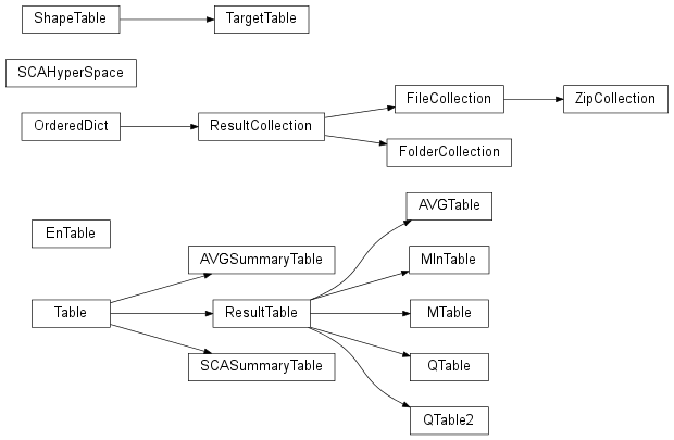
Table()	Base class for tables
ResultTable(fname, hdr_len, c_width[, ...])	Base class for results tables read from file.
AVGTable([fname, folder])	A class for reading .avg files.
AVGSummaryTable([fname, folder, npol, ...])	A class for reading the summary section of AVGTables.
SCASummaryTable([fname, folder, npol, zfile])	A class for reading the summary section of .sca files.
QTable([fname, folder])	A class for reading qtable output files.
QTable2([fname, folder])	A class for reading qtable2 output files.
MTable([fname])	A class for reading mtables output by DDSCAT.
MInTable([fname])	A class for reading material input files.
ShapeTable([fname, folder])	A class for reading shape.dat files.
TargetTable([fname, folder])	A class for reading target.out files.
EnTable([fname, folder, zfile])	Class for reading the .E1 and .E2 files from nearfield calcs.
ResultCollection()

Collection Classes

ResultCollection()
FolderCollection([r_type, path, recurse, fields])
FileCollection([r_type, path])
ZipCollection([r_type, folder])
SCAHyperSpace()	Create an object that stores the results from an isotropic simulation into a multi-dimensional np array.

Helper Functions

_dichroism_calculator(L, R)	Calculates the difference spectrum of two spectra.
split_string(s[, widths])	Splits a string into list of strings at the partition points provided by the sequence widths.
clean_string(s)	Remove illegal tokens from a string to return something appropriate for a Python name
Esq(E)	Return the magnitude squared of a vector field.

Class Definitions

For reading, manipulating and plotting the output files from DDSCAT

Results from an individual file (e.g. qtable or shape.dat) are held within a dictionary-like object. The columns of the table (e.g. wavelength, Q_ext) are accessible as entires in the dictionary that can be accessed using the key name (e.g. T[‘wave’], T[‘Q_ext’]). Other results parameters like polarization are available as attribute fields (eg. T.Epol). The available fields vary between result types.

The fields available as table columns can be found with T.keys(). The other attributes can be found with dir(T).

class ScatPy.results.AVGSummaryTable(fname=None, folder=None, npol=None, ncomps=None, zfile=None, **kwargs)

Bases: ScatPy.results.Table

A class for reading the summary section of AVGTables.

dichroism()

Calculate the dichroism

refresh()

Reload the data from the file.

class ScatPy.results.AVGTable(fname=None, folder=None, **kwargs)

Bases: ScatPy.results.ResultTable

A class for reading .avg files.

class ScatPy.results.EnTable(fname=None, folder=None, zfile=None)

Bases: dict

Class for reading the .E1 and .E2 files from nearfield calcs.

Parameters:

• fname – The name of the En file to load. Default is ‘w000r000k000.E1’.
• folder – The subfolder relative to CWD from which to load the table.
• zfile – The zipfile from which to load the table.

Results are returned as a dictionary of complex 3D numpy arrays. The key names corresponds to the following fields:

Comp: composition identifier at all points (0 for vacuum) Pol: polarization/d^3 at all points Esca: complex radiated E field at all points Einc: complex incident E field at all points Pdia: diagonal element of polarizability/d^3 at all pts Etot: The complex total E field at all points Etot2: The magnitude squared of the E field at all points

refresh()

Refresh the data from the file

set_folder(new_folder)

Change the working folder.

show(show_now=True, field=None)

Visualize the selected field with mayavi

Parameters:show_now – If True calls mlab.show immediately.

call mlab.show() to display the figure after making desired adjustments

ScatPy.results.Esq(E)

Return the magnitude squared of a vector field.

class ScatPy.results.FileCollection(r_type=None, path=None)

Bases: ScatPy.results.ResultCollection

dichroism(fields=None)

make_table()

Compile the various files into one table

split()

Split the collection into two collections corresponding to the two polarizations

class ScatPy.results.FolderCollection(r_type=None, path=None, recurse=True, fields=None)

Bases: ScatPy.results.ResultCollection

class ScatPy.results.MInTable(fname=None, **kwargs)

Bases: ScatPy.results.ResultTable

A class for reading material input files.

Simple file names are resolved relative to the default material_library path.

This class can be called to return an interpolated value at a requested wavelength. e.g.:

M=MInTable('Gold.txt')
refr_index=M(0.750)

refresh()

save(fname)

class ScatPy.results.MTable(fname=None, **kwargs)

Bases: ScatPy.results.ResultTable

A class for reading mtables output by DDSCAT.

Fields are: wave(um), f(cm-1), Re(m), Im(m), Re(eps), Im(eps)

class ScatPy.results.QTable(fname=None, folder=None, **kwargs)

Bases: ScatPy.results.ResultTable

A class for reading qtable output files.

Fields are: aeff, wave, Q_ext, Q_abs, Q_sca, g(1)=<cos>, <cos^2>, Q_bk, Nsca

class ScatPy.results.QTable2(fname=None, folder=None, **kwargs)

Bases: ScatPy.results.ResultTable

A class for reading qtable2 output files.

Fields are: aeff, wave, Q_pha, Q_pol, Q_cpol

class ScatPy.results.ResultCollection

Bases: collections.OrderedDict

dichroism(fields=None)

Calculate the dichroism between pairs of spectra.

Spectra are considered to form a pair if they come from folders with identical names suffixed with _cL and _cR (e.g. ‘sphere1_cL’ and ‘sphere2_cR’).

export(fields)

plot(fields=None, label=None, normalize=False, lw=2, **kwargs)

Plot all of the tables in the collection in one plot.

smooth(width=None, pad_sample=5)

class ScatPy.results.ResultTable(fname, hdr_len, c_width, folder=None, zfile=None)

Bases: ScatPy.results.Table

Base class for results tables read from file.

Parameters:

• fname – the file name, resolved relative to the `folder`
• hdr_len – The number of header lines to ignore.
• c_width – A list of column widths.
• folder – the subfolder from which to read the table. Default is the CWD.
• zfile – A zip archive from which to load the table.

Most DDscat output files have fixed column widths and cannot be relied upon to have whitespace between adjacent columns. Therefore the columns’ width must be provided in the c_width list.

Field names are derived from the column headings in the result table. The fields can be accessed like a Python dict, e.g. T[‘wave’]

refresh()

Reload the data from the file.

set_folder(new_folder)

Change the working folder.

class ScatPy.results.SCAHyperSpace

Create an object that stores the results from an isotropic simulation into a multi-dimensional np array.

The array indices correspond to:

[lambda, aeff, beta, theta, phi, Epol, Q]

In dichroism spectra there is no polarization dependance so the indices are:

[lambda, aeff, beta, theta, phi, CD]

The array is addressed by integer indices. The wavelength/radius/angle corresponding to a given index can be recoverred with he lists w_range, r_range, etc.

ProcessSCASpace()

Identify the extents of the dataset in w,r,k, and Epol

dichroism()

mean(*args, **kwargs)

refresh()

Load the sca data into the array

class ScatPy.results.SCASummaryTable(fname=None, folder=None, npol=None, zfile=None, **kwargs)

Bases: ScatPy.results.Table

A class for reading the summary section of .sca files.

dichroism()

Calculate the dichroism

refresh()

class ScatPy.results.ShapeTable(fname=None, folder=None)

Bases: dict

A class for reading shape.dat files.

copy()

refresh()

Refresh the data from the file

set_folder(new_folder)

Change the working folder.

show(show_now=True, *args, **kwargs)

Display the dipoles using Mayavi.

Parameters:show_now – If True calls mlab.show immediately.

Does not display dipole anisotropy.

class ScatPy.results.Table

Bases: dict

Base class for tables

Results from an individual file (e.g. qtable or shape.dat) are held within a dictionary-like object. The columns of the table (e.g. wavelength, Q_ext) are accessible as entires in the dictionary that can be accessed using the key name (e.g. T[‘wave’], T[‘Q_ext’]). Other results parameters like polarization are available as attribute fields (eg. T.Epol). The available fields vary between result types.

The fields available as table columns can be found with T.keys(). The other attributes can be found with dir(T).

Tables have attributes `x_field` and `y_fields` which indicate the default fields to use for the x axis and y axes when plotting.

copy()

Make a copy of the table

export(fname, fields=('Q_ext', ))

Export the table as an ascii file

Parameters:

• fname – The name of the file to be created.
• fields – The fields to save.

interpolate(n_pts=200)

Interpolates the data onto a new (denser) xrange.

Data is modified in place.

plot(y_fields=None, normalize=False, smooth=False, x_field=None, label=None, lw=2, **kwargs)

Plot the table contents.

Parameters:

• y_fields – list of field names to plot. If absent, plots the fields found in self.y_fields
• normalize – if True, set the maximum of all plots to 1
• smooth – if True, applies a spline smooth to the plot
• x_field – specify the field to plot as the x axis. Default is self.x_field
• label – a string giving a specific label for the y-axis

Returns:

the axes of the plot

scale(c)

Scale all fields of table by value c

Parameters:c – The value by which to scale.

smooth(width=None, pad_sample=5)

Broaden a spectrum by convolving with Gaussian

Spectrum is smoothed in place.

sig, signal w, FWHM

class ScatPy.results.TargetTable(fname=None, folder=None)

Bases: ScatPy.results.ShapeTable

A class for reading target.out files.

copy()

class ScatPy.results.ZipCollection(r_type=None, folder=None)

Bases: ScatPy.results.FileCollection

ScatPy.results.clean_string(s)

Remove illegal tokens from a string to return something appropriate for a Python name

ScatPy.results.dichroism_from_avg(fields, folder=None)

ScatPy.results.ellipticity_surf(DeltaQ, a_eff, rho)

Calculate the ellipticity in deg of a suspension

Parameters:

• DeltaQ – Q difference spectra.
• a_eff – the effective radius (in um).
• rho – the surface density in number/um^2.

ScatPy.results.ellipticity_vol(DeltaQ, a_eff, C, l=1)

Calculate the ellipticity in deg of a suspension

Parameters:

• DeltaQ – Q difference spectra.
• a_eff – the effective radius (in um).
• C – the concentration in mol/l.
• l – the pathlength in cm.

ScatPy.results.molar_ellipticity(DeltaQ, a_eff, C, l=1)

Calculate the molar ellipticity

Parameters:

• DeltaQ – Q difference spectra.
• a_eff – the effective radius (in um).
• C – the concentration in mol/l.
• l – the pathlength in cm.

ScatPy.results.plot_dichroism_from_avg(fields=None, lw=None, normalize=False, **kwargs)

ScatPy.results.split_string(s, widths=None)

Splits a string into list of strings at the partition points provided by the sequence widths.

Required to parse ddscat results files which are fixed width often without whitespace