\[\DeclareMathOperator{\erf}{erf} \DeclareMathOperator{\argmin}{argmin} \newcommand{\R}{\mathbb{R}} \newcommand{\n}{\boldsymbol{n}}\]

Parametric regression tutorial

Introduction

Given a set of observations \((x_i, y_i)\), with \(x_i = (x_{i1}, \ldots, x_{ip})^T \in \mathbb{R}^p\). We assume, there exists a function \(f(\theta, x)\) and a set of parameters \(\theta \in \mathbb{R}^q\) such that:

\[y_i = f(\theta, x_i) + \epsilon_i\]

with \(\epsilon_i \in \mathbb{R}\) such that \(E(\epsilon) = 0\).

The objective is to fine the set of parameters theta. Obviously, the real function is inaccesible. Instead, we will try to find an estimate of the parameters, \(\hat{\theta}\) using the least square estimator, which is:

\[\hat{\theta} = \argmin_{\theta \in \mathbb{R}^q} \left( f(\theta,x_i) - y_i \right)^2\]

The method is based on the SciPy function scipy.optimize.leastsq, which relies on the MINPACK’s functions lmdif and lmder. Both functions implement a modified Levenberg-Marquardt algorithm to solve the least-square problem. Most of the output of the main curve fitting option will be the output of the least-square function in scipy.

A simple example

As a simple example, we will take the function \(f\) to be:

\[f((a_0,a_1,a_2),x) = a_0 + a_1 x + a_2 x^2\]

Let’s assume the points look like this:

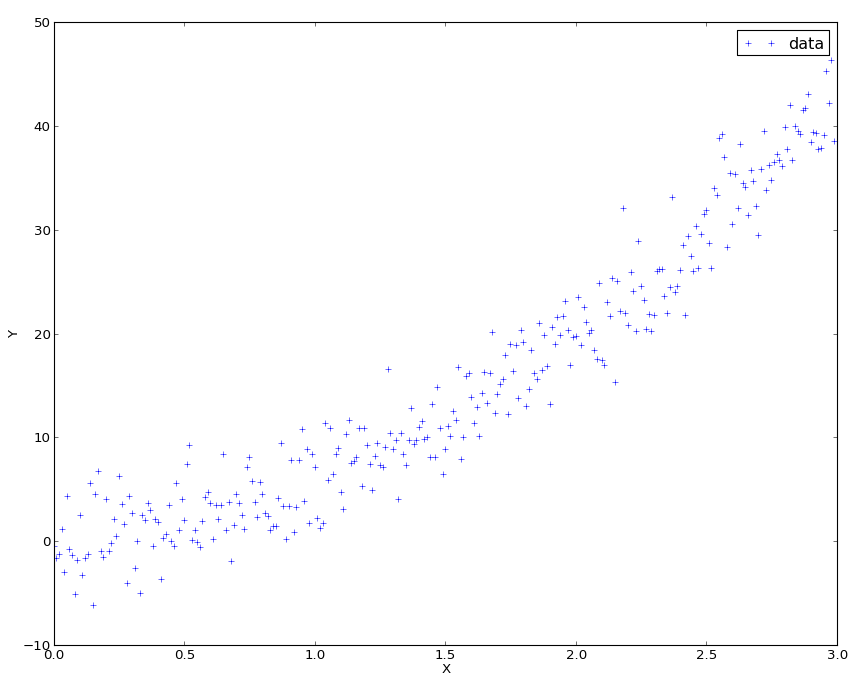
Raw data for curve fitting

The data points have been generated by that script:

>>> import numpy as np
>>> from matplotlib import pylab as plt
>>> x = np.arange(0,3,0.01)
>>> y = 2*x + 4*x**2 + 3*np.random.randn(*x.shape)
>>> plt.plot(x,y,'+',label='data')
>>> plt.legend(loc=0)
>>> plt.xlabel('X'); plt.ylabel('Y')

So we will expect to find something close to \((0,2,4)\).

To perform the analysis, we first need to define the function to be fitted:

>>> def f(params, x):
...   a0, a1, a2 = params
...   return a0 + a1*x+ a2*x**2

Then, we construct a CurveFitting object, which computes and stores the optimal parameters, and also behaves as a function for the fitted data:

>>> import pyqt_fit
>>> fit = pyqt_fit.CurveFitting(x,y,(0,1,0),f)
>>> print "The parameters are: a0 = {0}, a1 = {1}, a2 = {2}".format(*fit.popt)
The parameters are: a0 = 0.142870141922, a1 = 1.33420587099, a2 = 4.27241667343
>>> yfitted = fit(x)

The fit object, beside being a callable object to evaluate the fitting function as some points, contain the following properties:

fct

Function being fitted (e.g. the one given as argument)

popt

Optimal parameters for the function

res

Residuals of the fitted data

pcov

Covariance of the parameters around the optimal values.

infodict

Additional estimation outputs, as given by scipy.optimize.leastsq()

Fitting analysis

PyQt-Fit also has tools to evaluate your fitting. You can use them as a whole:

>>> from pyqt_fit import plot_fit
>>> result = plot_fit.fit_evaluation(fit, x, y,
...                                 fct_desc = "$y = a_0 + a_1 x + a_2 x^2$",
...                                 param_names=['a_0', 'a_1', 'a_2'])

You can then examine the result variable. But you can also perform only the analysis you need. For example, you can compute the data needed for the residual analysis with:

>>> rm = plot_fit.residual_measures(fit.res)

rm is a named tuple with the following fields:

scaled_res

Scaled residuals, sorted in ascending values for residuals. The scaled residuals are computed as \(sr_i = \frac{r_i}{\sigma_r}\), where \(\sigma_r\) is the variance of the residuals.

res_IX

Ordering indices for the residuals in scaled_res. This orders the residuals in an ascending manner.

prob

List of quantiles used to compute the normalized quantiles.

normq

Value expected for the quantiles in prob if the distribution is normal. The foluma is: \(\Phi(p) = \sqrt{2} \erf^{-1}(2p-1), p\in[0;1]\)

Plotting the results

At last, you can use the display used for the GUI:

>>> handles = plot_fit.plot1d(result)

What you will obtain are these two graphs:

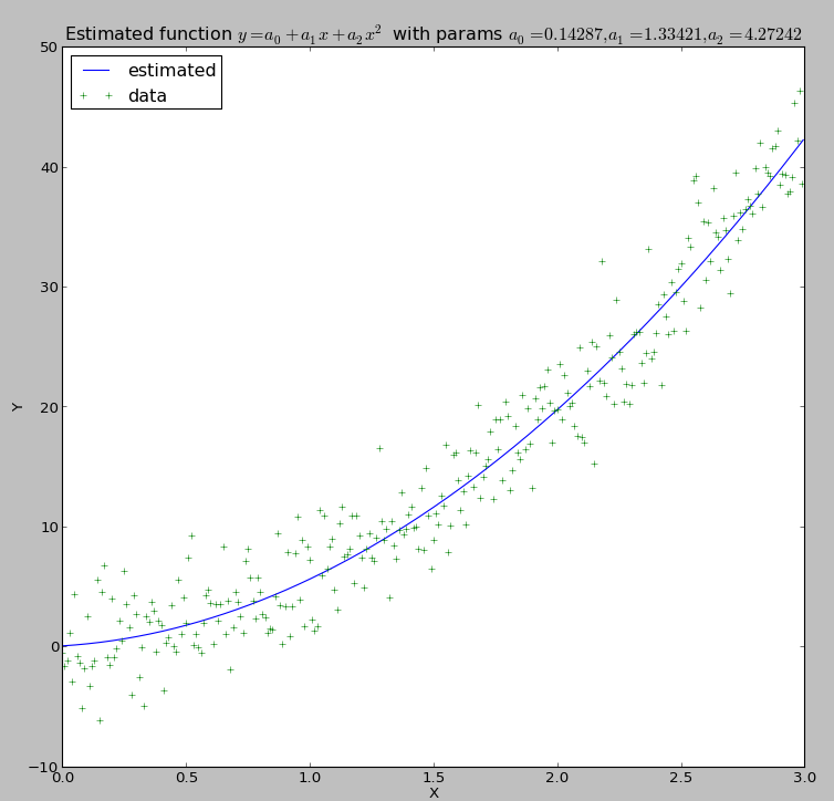
Curve fitting output

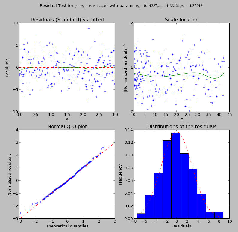
Residual checking output

Do not hesitate to look at the code for pyqt_fit.plot_fit.plot1d() to examine how things are plotted. The function should return all the handles you may need to tune the presentation of the various curves.

Speeding up the fitting: providing the jacobian

The least-square algorithm uses the jacobian (i.e. the derivative of the function with respect to each parameter on each point). By default, the jacobian is estimated numerically, which can be quite expensive (if the function itself is). But in many cases, it is fairly easy to compute. For example, in our case we have:

\[\begin{split}\begin{array}{rcl} \frac{\partial f(x)}{\partial a_0} &=& 1 \\ \frac{\partial f(x)}{\partial a_1} &=& x \\ \frac{\partial f(x)}{\partial a_2} &=& x^2 \end{array}\end{split}\]

By default, the derivatives should be given in columns (i.e. each line correspond to a parameter, each column to a point):

>>> def df(params, x):
...   result = np.ones((3, x.shape[0]), dtype=float)
...   result[1] = x
...   result[2] = x**2
...   return result # result[0] is already 1
>>> fit.Dfun = df
>>> fit.fit()

Of course there is no change in the result, but it should be slightly faster (note that in this case, the function is so fast that to make it worth it, you need a lot of points as input).

Confidence Intervals

PyQt-Fit provides bootstrapping methods to compute confidence intervals. Bootstrapping is a method to estimate confidence interval and probability distribution by resampling the data provided. For our problem, we will call:

>>> import pyqt_fit.bootstrap as bs
>>> xs = np.arange(0, 3, 0.01)
>>> result = bs.bootstrap(pyqt_fit.CurveFitting, x, y, eval_points = xs, fit_kwrds = dict(p0 = (0,1,0), function = f), CI = (95,99), extra_attrs = ('popt',))

This will compute the 95% and 99% confidence intervals for the curves and for the optimised parameters (popt). The result is a named tuple pyqt_fit.bootstrap.BootstrapResult. The most important field are y_est and CIs that provide the estimated values and the confidence intervals for the curve and for the parameters.

On the data, the result can be plotted with:

>>> plt.plot(xs, result.y_fit(xs), 'r', label="Fitted curve")
>>> plt.plot(xs, result.CIs[0][0,0], 'g--', label='95% CI')
>>> plt.plot(xs, result.CIs[0][0,1], 'g--')
>>> plt.fill_between(xs, result.CIs[0][0,0], result.CIs[0][0,1], color='g', alpha=0.25)
>>> plt.legend(loc=0)

The result is:

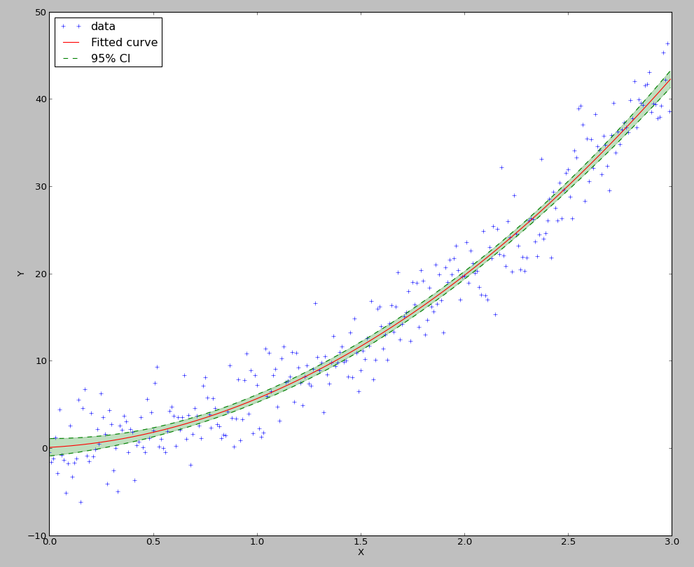
Drawing of the 95% confidence interval

The bounds for the parameters are obtained with:

>>> print "95% CI for p0 = {}-{}".format(*result.CIs[1][0])
>>> print "99% CI for p0 = {}-{}".format(*result.CIs[1][1])
95% CI for p0 = [-0.84216998 -0.20389559  3.77950689]-[ 1.14753806  2.8848943   4.7557855 ]
99% CI for p0 = [-1.09413524 -0.62373955  3.64217184]-[ 1.40142123  3.32762714  4.91391328]

It is also possible to obtain the full distribution of the values for the curve and for the parameters by providing the argument full_results=True and by looking at result.full_results.

Defining the functions and residuals

User-defined function

The function must be a two argument python function:

1. the parameters of the function, provided either as a tuple or a ndarray
2. the values on which the function is to be evaluated, provided as a single value or a ndarray

If the second argument is a ndarray of shape (...,N), the output must be a ndarray of shape (N,).

If is also possible to provide the function computing the Jacobian of the estimation function. The arguments are the same as for the function, but the shape of the output must be (P,N), where P is the number of parameters to be fitted, unless the option col_deriv is set to 0, in which case the shape of the output must be (N,P).

User-defined residuals

It is also possible to redefine the notion of residuals. A common example is to use the log of the residuals. It is most applicable if the standard deviation of the residuals is proportional to the fitted quantity. The residual should be a function of two arguments:

1. the measured data
2. the fitted data

For example, the log residuals would be:

>>> def log_residuals(y1, y0):
...   return np.log(y1/y0)

As for the user-defined function, it is possible to provide the jacobian of the residuals. It must be provided as a function of 3 arguments:

1. the measured data
2. the fitted data
3. the jacobian of the function on the fitted data

The shape of the output must be the same as the shape of the jacobian of the function. For example, if col_deriv is set to True, the jacobian of the log-residuals will be defined as:

>>> def Dlog_residual(y1, y0):
...   return -1/y0[np.newaxis,:]

This is because:

\[\mathcal{J}\left(\log\frac{y_1}{y_0}\right) = -\frac{\mathcal{J}(y_0)}{y_0}\]

as \(y_1\) is a constant, and \(y_0\) depend on the parameters.

Also, methods like the residuals bootstrapping will require a way to apply residuals on fitted data. For this, you will need to provide a function such as:

>>> def invert_log_residuals(y, res):
...   return y*np.exp(res)

This function should be such that this expression returns always true:

>>> all(log_residuals(invert_log_residuals(y, res), y) == res)

Of course, working with floating point values, this is usually not happening. So a better test function would be:

>>> sum((log_residuals(invert_log_residuals(y, res), y) - res)**2) < epsilon

Using the functions/residuals defined for the GUI

It is also possible to use the functions and residuals defined for the GUI. The interface for this are via the modules pyqt_fit.functions and pyqt_fit.residuals.

The list of available functions can be retrieved with:

>>> pyqt_fit.functions.names()
['Power law', 'Exponential', 'Linear', 'Logistic']

And a function is retrieved with:

>>> f = pyqt_fit.functions.get('Logistic')

The function is an object with the following properties:

__call__

Evaluate the function on a set of points, as described in the previous section

Dfun

Evaluate the jacobian of the function. If not available, this property is set to None

args

Name of the arguments

description

Formula or description of the evaluated function

init_args

Function provided a reasonnable first guess for the parameters. Should be called with f.init_args(x,y).

In the same way, the list of available residuals can be retrieved with:

>>> pyqt_fit.residuals.names()
['Difference of the logs', 'Standard']

And a residuals function is retrieved with:

>>> r = pyqt_fit.residuals.get('Difference of the logs')

The residuals is an object with the following properties:

__call__

Evaluate the residuals, as described in the previous section

Dfun

Evaluate the jacobian of the residuals. If not available, this property is set to None

invert

Function that apply the residuals to a set of fitted data. It will be called as r.invert(y, res). It should have the properties of the invert function described in the previous section.

description

Description of the kind of residuals

name

Name of the residuals.