\[\DeclareMathOperator{\erf}{erf} \DeclareMathOperator{\argmin}{argmin} \newcommand{\R}{\mathbb{R}} \newcommand{\n}{\boldsymbol{n}}\]

Regression using the GUI - tutorial

Using the interface

The script is starting from the command line with:

$ pyqt_fit1d.py

Once starting the script, the interface will look like this:

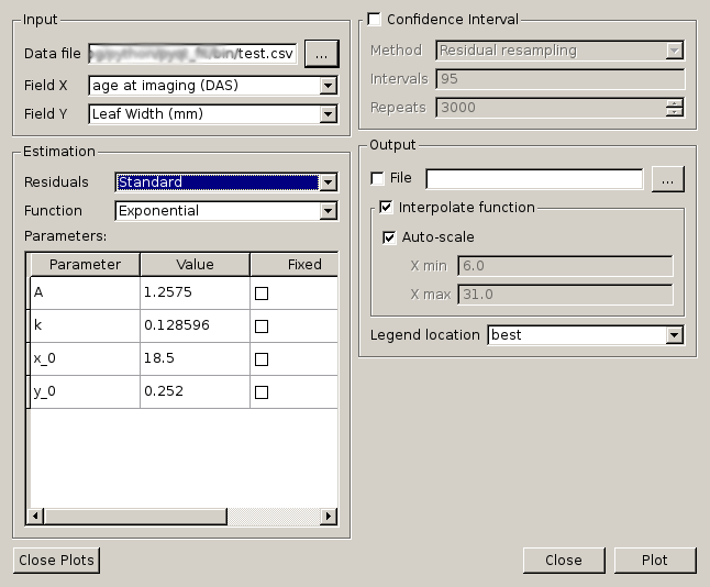
Main GUI of PyQt-Fit

The interface is organised in 4 sections:

1. the top-left of the window to define the data to load and process;
2. the bottom-left to define the function to be fitted and its parameters;
3. the top-right to define the options to compute confidence intervals;
4. the bottom-right to define the output options.

Loading the Data

The application can load CSV files. The first line of the file must be the name of the available datasets. In case of missing data, only what is available on the two selected datasets are kept.

Once loaded, the available data sets will appear as option in the combo-boxes. You need to select for the X axis the explaining variable and the explained variable on the Y axis.

Defining the regression function

First, you will want to choose the function. The available functions are listed in the combo box. When selecting a function, the list of parameters appear in the list below. The value presented are estimated are a quick estimation from the data. You can edit them by double-clicking. It is also where you can specify if the parameter is of known value, and should therefore be fixed.

If needed, you can also change the computation of the residuals. By default there are two kind of residuals:

Standard

residuals are simply the difference between the estimated and observed value.

Difference of the logs

residual are the difference of the log of the values.

Plotting and output

By default, the output consists in the data points, and the fitted function, interpolated on the whole range of the input data. If is, however, possible to both change the range of data, or even evaluate the function on the existing data points rather than interpolated ones.

The output also presents a window to evaluate the quality of the fitting:

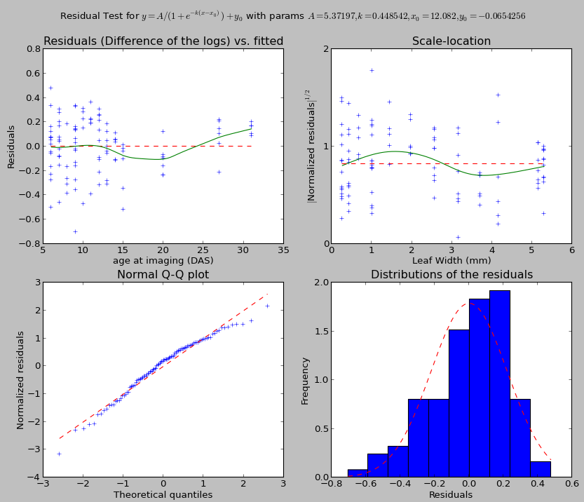
In general, the dashed red line is the target to achieve for a good fitting. When present the green line is the estimates that should match the red line.

The top-left graph presents the distribution of the residuals against the explaining variable. The green line shows a local-linear regression of the residuals. It should be aligned with the dashed red line.

The top-right graph presents the distribution of the square root of the standardized residuals against the explained variable. The purpose of this graph is to test the uniformity of the distribution. The green line is again a local-linear regression of the points. The line should be as flat and horizontal as possible. If the distribution is normal, the green line should match the dashed red line.

The bottom right graph presents a histogram of the residuals. For parametric fitting, the residuals should globally be normal.

The bottom left graph presents a QQ-plot, matching the theoretical quantiles and the standardized residuals. If the residuals are normally distributed, the points should be on the dashed red line.

The result of the fitting can also be output. What is written correspond exactly to what is displayed. The output is also a CSV file, and is meant to be readable by a human.

Confidence interval

Confidence interval can be computed using bootstrapping. There are two kinds of boostrapping implemented:

regular bootstrapping

The data are resampled, the pairs \((x,y)\) are kept. There is no assumption made. But is is often troublesome in regression, tending to flatten the results.

residual resampling

After the first evaluation, for each pair \((x,y)\), we find the estimated value \(\hat{y}\). Then, the residuals are re-sampled, and new pairs \((x,\hat{y}+r')\) are recreated, \(r'\) being the resampled residual.

The intervals ought to be a list of semi-colon separated values of percentages. At last, the number of repeats will define how many re-sampling there will be.

Defining your own function

First, you need to define the environment variable PYQTFIT_PATH and add a list of colon-separated folders. In each folder, you can add python modules in a functions sub-folder. For example, if the path ~/.pyqtfit is in PYQTFIT_PATH, then you need to create a folder ~/.pyqtfit/functions, in which you can add your own python modules.

Which module will be loaded, and the functions defined in it will be added in the interface. A function is a class or an object with the following properties:

name

Name of the function

description

Equation of the function

args

List of arguments

__call__(args, x)

Compute the function. The args argument is a tuple or list with as many elements are in the args attribute of the function.

init_args(x,y)

Function guessing some initial arguments from the data. It must return a list or tuple of values, one per argument to the function.

Dfun(args, x)

Compute the jacobian of the function at the points c. If the function is not provided, the attribute should be set to None, and the jacobian will be estimated numerically.

As an example, here is the definition of the cosine function:

import numpy as np

class Cosine(object):
  name = "Cosine"
  args = "y0 C phi t".split()
  description = "y = y0 + X cos(phi x + t)"

  @staticmethod
  def __call__((y0,C,phi,t), x):
    return y0 + C*np.cos(phi*x+t)

  Dfun = None

  @staticmethod
  def init_args(x, y):
    C = y.ptp()/2
    y0 = y.min() + C
    phi = 2*np.pi/x.ptp()
    t = 0
    return (y0, C, phi, t)

Defining your own residual

Similarly to the functions, it is possible to implement your own residual. The rediduals need to be in a residuals folder. And they need to be object or classes with the following properties:

name

Name of the residuals

description

Formula used to compute the residuals

__call__(y1, y0)

Function computing the residuals, y1 being the original data and y0 the estimated data.

invert(y, res)

Function applying the residual to the estimated data.

Dfun(y1, y0, dy)

Compute the jacobian of the residuals. y1 is the original data, y0 the estaimted data and dy the jacobian of the function at y0.

As an example, here is the definition of the log-residuals:

class LogResiduals(object):
  name = "Difference of the logs"
  description = "log(y1/y0)"

  @staticmethod
  def __call__(y1, y0):
    return log(y1/y0)

  @staticmethod
  def Dfun(y1, y0, dy):
    """
    J(log(y1/y0)) = -J(y0)/y0
    where J is the jacobian and division is element-wise (per row)
    """
    return -dy/y0[newaxis,:]

  @staticmethod
  def invert(y, res):
    """
    Multiply the value by the exponential of the residual
    """
    return y*exp(res)