Back to Guide
Building by aggregation
In pyny3d, everything is an aggregation of smaller objects. Even the lowest class, the Polygon, can be considered a sequence of points.
As it grows a 3D model its complexity increases, but if the general scheme is well understood, all the problems will be solved with a simple look to the documentation.
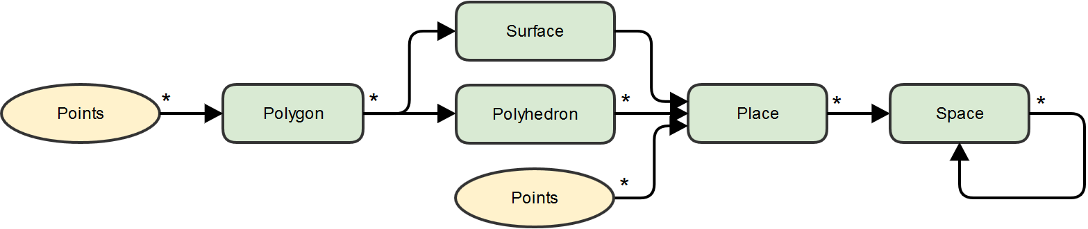
Simple Class Diagram (classes in green)
Multiple ordered Points form a Polygon. Multiple Polygons can form either a Surface or a Polyhedron. One Surface and multiple Polyhedra and Points form a Place. Multiple Places form a Space. And finally, an arbitrary number of Spaces can be aggregated to form a larger Space.
Classes initialization
First of all, we have to import the required packages:
import numpy as np
import pyny3d.geoms as pyny
In order to ease the call to the geoms module, it is convenient to
rename the whole sequence of pyny3d.geoms simply as pyny.
Polygon
Although this class represents a 3D polygon, it is important to remark that it
has to been planar and convex. By default, when a pyny.Polygon is
initialized, its convexity and counterclock wise orded is imposed
and when its parametric equation is required so is its planarity.
Polygons (doc: Polygon) can only be initialized using a ndarray where the columns are x, y, z coordinates and the rows are the ordered points that form the Polygon. This way, if we want to create a Polygon formed by the following points:
nº x y z 0 0 0 0 1 7 0 0 2 7 10 2 3 0 10 2
First, we have to create the ndarray and then initialize the pyny.Polygon
with it:
ordered_points = np.array([[0,  0, 0],
                           [7,  0, 0],
                           [7, 10, 2],
                           [0, 10, 2]])
polygon = pyny.Polygon(ordered_points)
At this point, we already have a ready-to-use pyny.Polygon. Probably, the
first thing you will want to do is to check it visually. To do so, you can
simply use the .plot() method that all classes have:
polygon.plot('b') # 'b' indicates blue color

Surface
A Surface (doc: Surface) is a group of contiguous Polygons. It is possible, depending on their distribution, that some methods work for a non-contiguous ones but it is very important to recall that the whole library has been developed under the hypothesis that they are. If you need to work with disperse groups of polygons, use multiple surfaces and englobe them in superior structures (Space).
To initialize a Surface, both a list of pyny.Polygons or a list of
ndarrays can be used. This two ways of initializing a Surface are identical:
# Polygon by Polygon (redundant)
polygon_0 = np.array([[0,0,0], [7,0,0], [7,10,2], [0,10,2]])
polygon_0 = pyny.Polygon(polygon_0)

polygon_1 = np.array([[0,10,2], [7,10,2], [3,15,3.5]])
polygon_1 = pyny.Polygon(polygon_1)

polygon_2 = np.array([[0,10,2], [3,15,3.5], [0,15,3.5]])
polygon_2 = pyny.Polygon(polygon_2)

polygon_3 = np.array([[7,10,2], [15,10,2], [15,15,3.5], [3,15,3.5]])
polygon_3 = pyny.Polygon(polygon_3)

surface_0 = pyny.Surface([polygon_0, polygon_1, polygon_2, polygon_2])


# Simultaneously (clearer)
polygons_list = [np.array([[0,0,0], [7,0,0], [7,10,2], [0,10,2]]),
                 np.array([[0,10,2], [7,10,2], [3,15,3.5]]),
                 np.array([[0,10,2], [3,15,3.5], [0,15,3.5]]),
                 np.array([[7,10,2], [15,10,2], [15,15,3.5], [3,15,3.5]])]
surface_0 = pyny.Surface(polygons_list)
As we did before, the best way to verify the Surface is to plot it:
surface_0.plot('b')

As you can see in the figure above, the Surface is actually a composition of two rectangles and one of them is, at the same time, a composition of two triangles and a trapezium. It is possible in pyny3d to melt the polygons which are complanars and contiguous at initialization of a Surface by:
surface_0 = pyny.Surface(polygons_list, melt=True)
surface_0.plot('b')
Melting multiple polygons can speedup heavy calculations (specially at
shading) and makes easier handle the geometries. On the other hand, make sure
that you previosly undertand the .melt() limitations
(doc: Surface).
Polyhedron
Polyhedron (doc: Polyhedron) represents 3D polygon-based convex Polyhedra. It is initialized by the polygons which form its faces in a very similar way as the Surface does:
faces_list = [np.array([[7,3,5], [7,0,5], [7,0,0],   [7,3,0.6]]),
              np.array([[7,0,5], [4,0,7], [4,0,0],   [7,0,0]]),
              np.array([[4,0,7], [4,3,7], [4,3,0.6], [4,0,0]]),
              np.array([[4,3,7], [7,3,5], [7,3,0.6], [4,3,0.6]]),
              np.array([[7,0,0], [4,0,0], [4,3,0.6], [7,3,0.6]]),
              np.array([[7,0,5], [4,0,7], [4,3,7],   [7,3,5]])]
polyhedron_0 = pyny.Polyhedron(faces_list)
polyhedron_0.plot('b')

Initialize Polyhedra this way is very verbose because given information is redundant about the faces. A far more convenient way to introduce a Polyhedron is by giving just the top and the bottom Polygons and telling the class that a connection between them is needed:
bottom = np.array([[7,0,5], [4,0,7], [4,3,7], [7,3,5]])
top =    np.array([[7,0,0], [4,0,0], [4,3,0.6], [7,3,0.6]])
polyhedron_0 = pyny.Polyhedron.by_two_polygons(top, bottom)
Both Polyhedra created are exactly the same one. Finally, it exists a better
way to create new Polyhedra by extruding a Polygon from a given position
to a Surface, what it is called “extruded obstacles”. The method
.add_extruded_obstacles() is in the Place class due to Surfaces, and
Polyhedra are aggregated there.
Thanks to these, you will probably never need to use the polygon_list initialization.
Place
Places (doc: Place) are initialized giving a Surface, a list of Polyhedra and a Set of Points but, actually, the only indispensable one is the Surface.
If we already have created the necessary objects, then we can use this simple way:
place_0 = pyny.Place(surface_0, polyhedron_0)
place_0.plot('b')

A Place can also be created giving directly the polygons that form its surface:
place_0 = pyny.Place(polygons_list, polyhedron_0)
The Place class is a dynamic one. It was conceived to be easily edited once
created with methods like .mesh() or .add_extruded_obstacles():
wall_1 = np.array([[0,0,4],    [0.25,0,4],  [0.25,15,4], [0,15,4]])
wall_2 = np.array([[0,14.7,5], [15,14.7,5], [15,15,5],   [0,15,5]])
place_0.add_extruded_obstacles([wall_1, wall_2])
place_0.mesh(0.5)   # distance between points
place_0.plot('b')

Adding points is possible by independently generate and inserting them
through .add_set_of_points() but if you want to simply create a regular
distributed set it is easier to use .mesh().
Space
Space (doc: Space) does not bring any new concept, it is only an aggregation of Places with the goal of being a container that makes possible global transformations with very few commands. As Place, Space is a dynamic class which has a lot of methods to interactively use it. For this reason, it is possible to build a Space through several ways.
The first and simplest way to create a Space is by giving it a list of Places as argument:
poly_surf = np.array([[8,0,0], [15,0,0], [15,9,0], [8,9,0]])
place_1 = pyny.Place(poly_surf)
space = pyny.Space([place_0, place_1])
Furthermore, it can be initialized empty and the elements can be added later:
space = pyny.Space()
space.add_places([place_0, place_1])
Combining multiple Spaces is as simple as:
space = pyny.Space(place_0)
space_1 = pyny.Space(place_1)
space.add_spaces(space_1)
All these code snippets create the same result:

Note that the place_0 has brought the set of points with it while the new
place (place_1) has not any point declared. If a more uniformed set of
points is required the easiest way is to clear the old and create a new one:
space.clear_sets_of_points()
space.mesh(0.5)
space.iplot(c_poly='b')

In short
All the steps above can be written just in five lines to generate exactly the last output:
import numpy as np
import pyny3d.geoms as pyny

# Declaring the geometry
## Surface
poly_surf_0 = [np.array([[0,0,0], [7,0,0], [7,10,2], [0,10,2]]),
               np.array([[0,10,2], [7,10,2], [3,15,3.5]]),
               np.array([[0,10,2], [3,15,3.5], [0,15,3.5]]),
               np.array([[7,10,2], [15,10,2], [15,15,3.5], [3,15,3.5]])]
poly_surf_1 = [np.array([[8,0,0], [15,0,0], [15,9,0], [8,9,0]])]

## Obstacles
wall_1 = np.array([[0,0,4], [0.25,0,4], [0.25,15,4], [0,15,4]])
wall_2 = np.array([[0,14.7,5], [15,14.7,5], [15,15,5], [0,15,5]])
chimney = np.array([[4,0,7], [7,0,5], [7,3,5], [4,3,7]])

# Building the solution
place_0 = pyny.Place(poly_surf_0, melt=True)
place_0.add_extruded_obstacles([wall_1, wall_2, chimney])
place_1 = pyny.Place(poly_surf_1)
space = pyny.Space([place_0, place_1])
space.mesh(0.5)

# Viz
space.iplot(c_poly='b')
Next tutorial: Classes usage