init=’auto’¶

When we set the init parameter in space.shadows() as ‘auto’, what we are technically declaring is: “I don’t care about the .arg_ parameters or whether the Space has points declared or not, just fill them all as you want and generate a sample simulation”. Obviously, you will not have a “true time” solution this way.

However, this initialization will let you introduce the following parameters (but will not obligate):

• data
• t
• dt
• latitude

Even, it will respect the Space’s set of points, if it exists. Here we can see an example:

In [4]: space_copy = space.copy()
   ...: space_copy.clear_sets_of_points()
   ...: space_copy[0].mesh(0.6)  # Points only in place #1
   ...: 

In [5]: S = space_copy.shadows(init='auto', dt=120, latitude=0.001)
   ...: S.viz.exposure_plot()
   ...: 

To make our life easier, we can adjust the simulations in 'auto' mode with the resolution argument. This also affects the time vector generated and the Voronoi’s diagram mesh size.

In [6]: space.clear_sets_of_points()

In [7]: space_copy = space.copy()
   ...: space_copy.shadows(init='auto', resolution='low').viz.exposure_plot()
   ...: 

In [8]: space_copy = space.copy()
   ...: space_copy.shadows(init='auto', resolution='mid').viz.exposure_plot()
   ...: 

In [9]: space_copy = space.copy()
   ...: space_copy.shadows(init='auto', resolution='high').viz.exposure_plot()
   ...: 

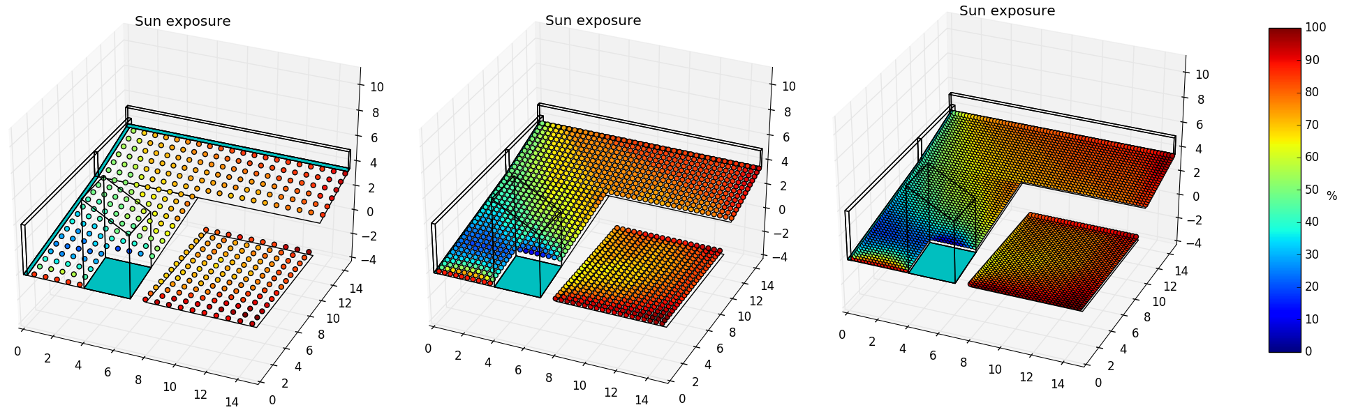
Visualization for the low, mid and high resolution. The execution time was 443 ms, 1.12 s and 3.58 s respectively.

The solution¶

pyny3d was created to work as a complement for larger applications. Until now, we have seen how to insert data, work with them and perform simulations. The next step is: “how and where is the simulation’s solution?”.

The answer is that it is a numpy array (surprise) that stores the ON/OFF state of each sensible point in each instant indicated in t. This array is in ShadowManager.light and its rows correspond to the t instants while its columns matches the points in the Space. For this example, we have computed 614 intervals for 4184 sensible points:

In [10]: S.light
Out[10]: 
array([[ True,  True,  True, ...,  True,  True,  True],
       [ True,  True,  True, ...,  True,  True,  True],
       [ True,  True,  True, ...,  True,  True,  True],
       ...,
       [ True,  True,  True, ..., False, False, False],
       [ True,  True,  True, ...,  True,  True,  True],
       [ True,  True,  True, ...,  True,  True,  True]], dtype=bool)

In [11]: S.light.shape
Out[11]: (614, 4184)

Note that for real computations where you probably have samples each 15 or 30 minutes, the number of rows will increase to 17500 - 35000.

On the other side, there is another version of the solution called light_vor stored in ShadowsManager.light_vor. In this case, the rows are the Voronoi’s diagram’s polygons, that is, the ON/OFF state of each point is referenced directly to the Solar Horizont discretization. Remember that each polygon of this discretization contains multiple (azimuth, zenit) pairs from the t and data vector.

In [12]: S.light_vor.shape
Out[12]: (277, 4184)

As we can see, the simulation has been made for 277 Sun positions that englobes the total 614 samples. However, if we run a simulation with a dt parameter considerably shorter the difference will be also considerably larger:

In [13]: S = space.shadows(init='auto', dt=15, resolution='high')

In [14]: S.light.shape  # 35040 samples in t
Out[14]: (35040, 4184)

In [15]: S.light_vor.shape  # 1139 polygons in the Voronoi's diagram
Out[15]: (1139, 4184)

In the next section we will see how we can control more specifically the parameters in order to generate more adjuted solutions, avoiding wasting resources.

Solar Horizont discretization¶

Finally, we are going to see a comparison between a coarse discretization and a much finer one.

The following visualizations are:

1. vor: Voronoi diagram of the Solar Horizont. Samples in blue, polygon

   centroinds in red. Polygons in semi-transparent blue.

2. data: Accumulated time integral of the data projected

   in the Voronoi diagram of the Solar Horizont.

3. freq: Frequency of Sun positions in t in the Voronoi

   diagram of the Solar Horizont.

In [16]: # Coarse discretization
    ...: S1 = space.shadows(init='auto', dt=856, resolution='mid')
    ...: S1.viz.vor_plot('vor')
    ...: S1.viz.vor_plot('data')
    ...: S1.viz.vor_plot('freq')

This simulation has 615 samples, and the discretization has 236 polygons. It took 2.58 s.

In [17]: # Fine discretization
    ...: S2 = space.shadows(init='auto', dt=13, resolution='mid')
    ...: S2.viz.vor_plot('vor')
    ...: S2.viz.vor_plot('data')
    ...: S2.viz.vor_plot('freq')

This simulation has 40431 samples, and the discretization has 479 polygons. It took 5.35 s.

It is very clear that the discretization avoids the simulation to last 66 times longer for the second one, even when it has 66 times more samples. Instead of this, it groups the samples by proximity, and consequently, the execution time, which depends only to the number of polygons, is homogenized.

The correspondant exposure_plots for the previous examples are:

As you can see, the visualization is in practice the same but, as we have seen, the problem have been solved with different time resolutions. Does this mean that the solution is exactly the same? Of course not. If you have some pyny3d processes inside a larger software processing, for example photovoltaic electric generation, I am sure that you prefer to know the ON/OFF state of the solar cells each quarter hour than each 14 hours, even the visualization where a year is summed up looks the same.

Next tutorial: Advanced shading tutorial