Keres Documentation
Keres is the testing suite for a Bayes filter useful for amyloid fibrillogenesis fluorimetry data.
The keres homepage is at <https://pypi.python.org/pypi/keres/> and the most complete documentation is available at <http://pythonhosted.org/keres/>.
Fibrillogenesis
Fibrillogenesis is the process of fiber formation by amyloid forming proteins, such as the Alzeimer’s protein A-beta. At the beginning of a fibrillogensis experiment, the total protein exists in a fiber-free form. After some time, the protein starts to form fibers in a rapidly accelerating reaction that eventually converts all of the protein to fibers.
The moment at which the first fibers are detected is the point of transition from the “lag phase” of no fibers to the “signal phase” where fibers are present. The “signal phase” gets its name from the fact that the fibers produce signal measureable by a detector. The time from the start of the experiment to the point of transition to the signal phase is called the “lag time”.
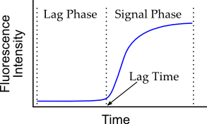
Schematized representation of fluorometric fibrillogenesis data.
Data is generally noisy, although this latter figure represents data as a smooth curve. The detector measures the light emitted from dyes that fluoresce when bound to amyloid fibers and irradiated at specific wavelengths. Thus, the continuous curve represents a series of many individual datapoints taken closely together.
Several problems with data, such as noisiness, incompleteness, or baseline drift make it difficult to measure the lag time with certainty. One way to address these challenges is to embrace this uncertainty and convert the series of intensities to a series of probabilities using a Bayes filter.
The Bayes Filter
The Bayes filter is an application of recursive Bayesian estimation, a full description of which will be published soon. But briefly, the principle of recursive Bayesian estimation is to update a posterior probability \(p_i(H|E)\), where \(i\) indexes the data point in a series. The probability \(p_i(H|E)\) describes how likely it is that the experiment is still in the lag phase of fibrillogenesis.
If the point \(i+1\) has higher signal than point \(i\), then \(p_i(H|E)\) gets lower (i.e. less likelihood that the experiment is still in the lag phase). Conversely, if the point \(i+1\) has lower signal than point \(i\), then \(p_i(H|E)\) gets higher.
For each round, the estimator is updated according to Bayes’s equation:
The value \(p_i(H)\) is the equal to \(p_{i-1}(H|E)\). The value \(p_i(E|H)\) is the probability to see a point with intensity \(I_i\) given that the experiment is in the lag phase. \(p_i(E|H)\) assumes a normal distribution of intensities around the mean intensity of the presumed lag phase (basically a reasonable window of data points prior to point \(i\)).
The value \(p_i(E)\) is the probability of seeing the intensity \(I_i\) in a reasonable window of points around point \(i\).
Once the probability \(p_i(H|E)\) falls below a hard cutoff (\(10^{-10}\)), the experiment is confidently in the signal phase.
To find the exact transition from the lag to signal phases, it is useful to “backtrack” to a higher probability (\(10^{-4}\)) and then apply an empircal correction optimized from simulation data with Gaussian noise:
Here, \(\nu_h\) is the average intensity around the hard cutoff point \(h\), \(\sigma_h\) is the square root of the variance of the lag phase for data point \(h\). The rest of the values are empirical: \(k = 7\), \(m = 362\), \(\alpha = 0.9\). Although this correction works well for both simulated and experimental data, we don’t have a rigorous theoretical rationale for its efficacy. In other words, this correction is entirely empirical.
Using the Bayes Filter Directly
Data can be passed to the default Bayes filter by calling the bayesian_pickup() function (“pickup” refers to when the signal “picks up”):
from keres import bayesian_pickup

(time, value), history, signoise = bayesian_pickup(data)
Here, data is a \(2 \times N\) array, where the first element is a vector of times (\(t_0, t_1, t_2 ... N\)) and the second element is a vector of intensities (\(I_0, I_1, I_2 ... N\)).
Return Values
The return value of bayesian_pickup() is a tuple of three elements, the first of which is a 2-tuple of the time at the end of the lag phase (“pickup”) and the intensity (value) at the pickup.
The second element, history, is a list of 2-tuples, each having a first element of the data point number \(i\) and a second element of the \(\log_{10} p_i(H|E)\):
Here, \(K\) is the number of data points in the lag phase.
The third element, signoise, is the ratio of the interpolated value (\(I_H\)) at the time \(t_H\) where \(p(H|E) = 10^{-10}\) to the standard deviation (\(\sigma_{j<i}\)) of the values \(j<i\) in the lag phase (all intensity values \(I_j\) prior to point \(i\)):
Example
As an example, let’s first simulate some data, using noise from a normal distribution:
from numpy import arange, array, vectorize
from numpy import random as rnd

size = 1000
lag = 200
scale = 5.0
noise = rnd.normal  # others could be rnd.exponential, rnd.poisson

curve = lambda i: -scale / (1 + (lag * max((i - lag) / size, 0)**2))

X = arange(size, dtype=float)
Y = map(curve, X) + noise(size=size)
data = array([X, Y - min(Y)])
To take a look at the data, we’ll plot it with pygmyplot:
from pygmyplot import xy_plot

figsize = (4, 2.5)
margins = {"bottom": 0.2, "left": 0.15, "right": 0.9}

norm_plot = xy_plot(*data, figsize=figsize)
norm_plot.axes.set_xlabel("time")
norm_plot.axes.set_ylabel("fluorescence intensity")
norm_plot.axes.figure.subplots_adjust(**margins)
norm_plot.refresh()
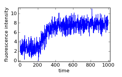
Simulated fibrillogenic data with normally distributed noise.
That data is plenty noisy. Let’s see how the Bayes filter, bayesian_pickup(), handles it:
from keres import bayesian_pickup
(time, value), history, signoise = bayesian_pickup(data)
print "time: %s,  value: %s" % (time, value)
For this random data, the latter command reports “time: 215.0, value: 3.11276048316”, meaning that filter decided that the lag time is 215.0 s. Let’s take a look at a zoom of the area:
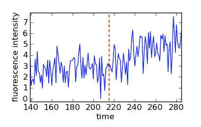
Zoom of simulated data with a vertical line at the measured lag time (t=215).
Clearly, bayesian_pickup() got very close to what a human might decide for this particular random data. Note that the actual lag time of the simulation is 200 s, defined by the line lag = 200.
This decision includes the correction described in Equation (2), but it is possible to see how the filter decided that the data had entered the signal phase by plotting the history element returned by bayesian_pickup():
history_plot = xy_plot(*array(history).T, figsize=figsize,
                                          sibling=norm_plot)
history_plot.axes.set_xlabel("time")
history_plot.axes.set_ylabel("$\log_{10}\{p_i(H|E)\}$ | Intensity")
history_plot.axes.set_xlim(0, 1000)
history_plot.refresh()
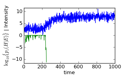
Bayes filter history (green) with simulated data (blue).
Here, the data (“Intensity”) and history (\(\log_{10}\{p_i(H|E)\}\)) curves are stacked. Y-lables for both are on the left hand side of the plot.
Following is a zoom of the history and data.
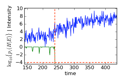
Zoom of Bayes filter history (green) with simulated data (blue).
The dashed lines in this figure show the “backtrack” point where \(p(H|E) = 10^{-4}\). Although it seems like the Bayes filter has picked a point too far into the signal phase, in actuality, the Bayes filter found the first point that peeks just above the noise. The following figure, which includes no points past 238 s, makes this fact clear:
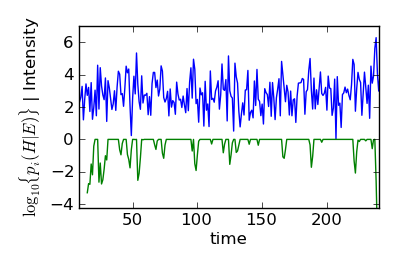
Bayes filter history (green) with simulated data (blue) for all times less than 238 s.
Using the Test Suite
Keres includes a testing suite accessible through the program bayestest, which is controlled by a configuration (“config”) file:
bayestest configfile
The config file has a number of settings, an example of which is in the examples folder of the source distribution. The example config file, settings.cfg, documents the settings as comments. Given a complete source distribution, it is possible to run bayestest without installing by issuing the following command from within the examples folder:
./test-bayes settings.cfg
Running bayestest as above will invoke the simulator to produce a specified number (plot_n) of plots that show individual simulations (not all simulations are necessarily plotted). The top panel of which will show the simulated noisy data in blue and the “noiseless” data superposed in green. The bottom pannel shows the history of the probability \(p(H|E)\):
Plot of simulated data (top) and history of \(p(H|E)\).
During the simulation, a report window is updated with information about the simulations and the performance of the various methods to measure lag time:
=======================================================
 Noise: 0.1
=======================================================
   real tenth  half bayes  diff
=======================================================
    234     0   259   231    -3
    291     0   313   285    -6
    252     0   274   247    -4
    420     0   438   412    -8
    367     0   390   360    -7
=======================================================
    312     0   335   307    -5

=======================================================
   Scaling N: 5,  Stocastic n: 2
   Length: 500,  Noise: 0.1
=======================================================
         10%|         50%|    Bayesian
=======================================================
  0.00164648|  0.88912049|  0.90321512 | KS p(Exponential)
107929.561885|   53.923670|   46.500000 | Variance
=======================================================
In this report, “Noise:” indicates the noise level as a fraction of the maximum signal for the noiseless data. The following table indicates the lag time for noiseless data (“real”), and the lag time found for each of the tenth-time, half-time, and Bayesian methods. The difference between the lag time as measured by the Bayesian method and the ‘real” time is given as “diff”. Means for each value are given in the bottom row of the table.
The second table reports number of different simultions ran for the noise level (in the above table, the number of simulations is \(10 = \mbox{Scaling N} \times \mbox{Stochastic n}\). The length of the data series (minus a randomly produced extension of the lag time) is given, along with the noise level as decribed above.
This table reports the p-value given by the K-S test for an exponential distribution on the lag time distributions, as measured by the three methods. For example, the p-value for the distribution of lag times measured by the Bayesian method is 0.903. The bottom row of this table reports the mean squared difference (MSD) of these distributions relative to the “real” lag time (\(t_r\)) of the simulation: