Backends

A backend is an implementation of a consistent interface, which provides basic operations for filtering N-dimensional arrays. These include filtering operations that build selectivity, pooling operations that build invariance, and an operation providing local contrast enhancement of an image.

Filtering

Four filter operations are supported. The operation DotProduct compares the input neigborhood and the weight vector (i.e., prototype) using a dot product, where each output is given by

\[y = X^T W\]

for input neighborhood \(X\) (given as a vector) and weight vector \(W\), where \(X^T\) denotes the matrix transpose. The operation NormDotProduct is similar, but constrains each vector to have unit norm. Thus, the output is given by

\[y = \text{NDP}(X, W) = \frac{X^T W}{\left\Vert X \right\Vert \left\Vert W \right\Vert} \, ,\]

where \(\left\Vert \cdot \right\Vert\) denotes the Euclidean norm.

Instead of a dot product, the operation Rbf compares the input and weight vectors using a radial basis function (RBF). Here, the output is given as

\[y = \exp \left\{ - \beta \left\Vert X - W \right\Vert ^2 \right\} \, ,\]

where \(\beta\) controls the sensitivity of the RBF. Constraining the vector norm of the arguments gives the final operation NormRbf, where the output is given as

\[y = \exp \left\{ - 2\beta \left(1 - \text{NDP}(X, W) \right) \right\} \, ,\]

Here, we have used the bilinearity of the inner product to write the distance as

\[\left\Vert V_a - V_b \right\Vert ^2 = 2 - 2 V_a^T V_b\]

for unit vectors \(V_a\) and \(V_b\).

Pooling

Currently, the only operation that is supported is a maximum-value pooling function. For a local neighborhood of the input \(X\), this computes an output value as

\[y = max_{i,j} \ x_{ij} \ .\]

This has been argued to provide a good match to cortical response properties [1], and has been shown in practice to lead to better performance [2].

Contrast Enhancement

Given a local input neighborhood \(X\), the output is

\[y = \frac{x_c - \mu}{\max(\sigma, \epsilon)}\]

where \(x_c\) is the center of the input neighborhood, \(\mu\) and \(\sigma\) are the mean and standard deviation of \(X\), and \(\epsilon\) is a bias term. Thus, we measure the local deviation from the mean, where large deviations are squashed if the window contains a large amount of variance.

The bias term is used to avoid the amplification of noise, and to ensure a non-zero divisor. Without the bias term, this method performs badly on homogeneous regions, where the variance approaches zero. In this case, very small local deviations (usually caused by image noise) become enhanced when the value of the denominator drops below unity. Because of this bias term, we will never enhance deviations, only “squash” them. This removes the noise in the background while retaining contrast enhancing effects of the foreground. This is illustrated below.

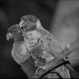
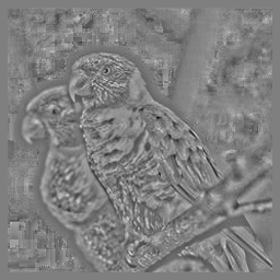
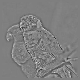
Original image.	Contrast enhancement.	Biased contrast enhancement.

References

[1]	Serre, T., Oliva, A. & Poggio, T., 2007. A feedforward architecture accounts for rapid categorization. Proceedings of the National Academy of Sciences, 104(15), p.6424-6429.

[2]	Boureau, Y.-L. et al., 2010. Learning mid-level features for recognition. In Computer Vision and Pattern Recognition 2010. IEEE, pp. 2559-2566.