Flattening Images with Step Edges

In this example you learn (again) how to open a demo image, how to display a image with and without a mask and how to flatten an image with step edges which does not have molecular or atomic resolution. Finally, you will learn how to create a histogram of the pixel heights to determine the difference in height between the terraces. For flattening the following functions are suitable:

• flatten_poly_xy() (only first order and without a mask)
• flatten_xy()

For locating step edges in an image:

• locate_steps()

Tutorial Example

Open a Python shell session and import the modules spiepy and spiepy.demo, list the available demo images in SPIEPy:

>>> import spiepy, spiepy.demo
>>> demos = spiepy.demo.list_demo_files()
>>> print demos
{0: 'image_with_defects.dat', 1: 'image_with_step_edge.dat', 2: 'image_with_step_edge_and_atoms.dat'}
>>>

Open the demo image image_with_step_edge.dat and display the image:

>>> im = spiepy.demo.load_demo_file(demos[1])
>>> import matplotlib.pyplot as plt
>>> plt.imshow(im, cmap = spiepy.NANOMAP, origin = 'lower')
<matplotlib.image.AxesImage object at 0x0424A150>
>>> plt.show()

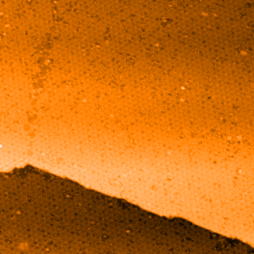
The standard colormap used by most SPM software is the orange colormap NANOMAP. The variable im is the original demo image. Before trying to locate the step edge, remove the tilt on the surface as much as possible. This improves the contrast of the step. Only first order polynomial planes should be used as higher order polynomials will try to fit the step. Either the function flatten_poly_xy() or flatten_xy() can be used to do this. Now flatten the image with the function flatten_xy():

>>> im_flat, _ = spiepy.flatten_xy(im)

The variable im_flat contains the flattened image, it is the input image minus fitted plane. im is not overwritten, the data will be flattened again later and it is best to avoid cumulative flattening where possible. The flattened image looks like:

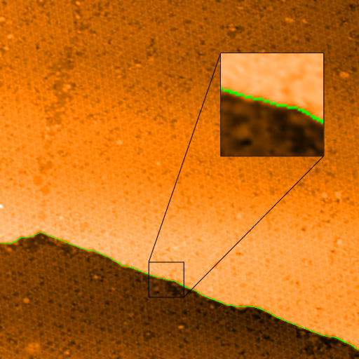
Clearly by looking at the top terrace there is a gradient on the sample, this is because the flattening routines do not work well when there is a step. By masking step edges the flattening function flatten_xy() can do the job. Find the step edges with the function locate_steps() and display the flattened image with the mask:

>>> mask = spiepy.locate_steps(im_flat, 4)
>>> palette = spiepy.NANOMAP
>>> palette.set_bad('#00ff00', 1.0)
>>> import numpy as np
>>> plot_image = np.ma.array(im_flat, mask = mask)
>>> plt.imshow(plot_image, cmap = palette, origin = 'lower')
<matplotlib.image.AxesImage object at 0x03127450>
>>> plt.show()

Once the step edges has been successfully located, the image can be re-flattened with the function flatten_xy(). Flatten the original image again using the keyword argument mask and the variable mask:

>>> im_final, _ = spiepy.flatten_xy(im, mask)

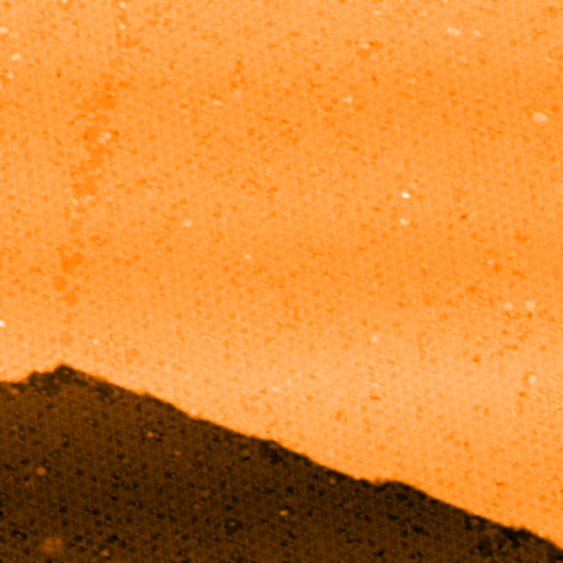
It is clear that each terrace is now free of its gradient. A final check which can be applied is to plot a histogram of the pixel heights. Create a histogram of the pixel heights for the images im_flat and im_final:

>>> y, x = np.histogram(im_flat, bins = 200)
>>> ys, xs = np.histogram(im_final, bins = 200)
>>> fig, ax = plt.subplots()
>>> ax.plot(x[:-1], y, '-b', label = 'Standard plane flattening')
[<matplotlib.lines.Line2D object at 0x04236AD0>]
>>> ax.plot(xs[:-1], ys, '-r', label = 'SPIEPy stepped plane flattening')
[<matplotlib.lines.Line2D object at 0x04236150>]
>>> ax.legend(loc = 2, fancybox = True, framealpha = 0.2)
<matplotlib.legend.Legend object at 0x04236C30>
>>> ax.set_xlabel('z (nm)')
<matplotlib.text.Text object at 0x04269CD0>
>>> ax.set_ylabel('count')
<matplotlib.text.Text object at 0x0423D330>
>>> plt.show()

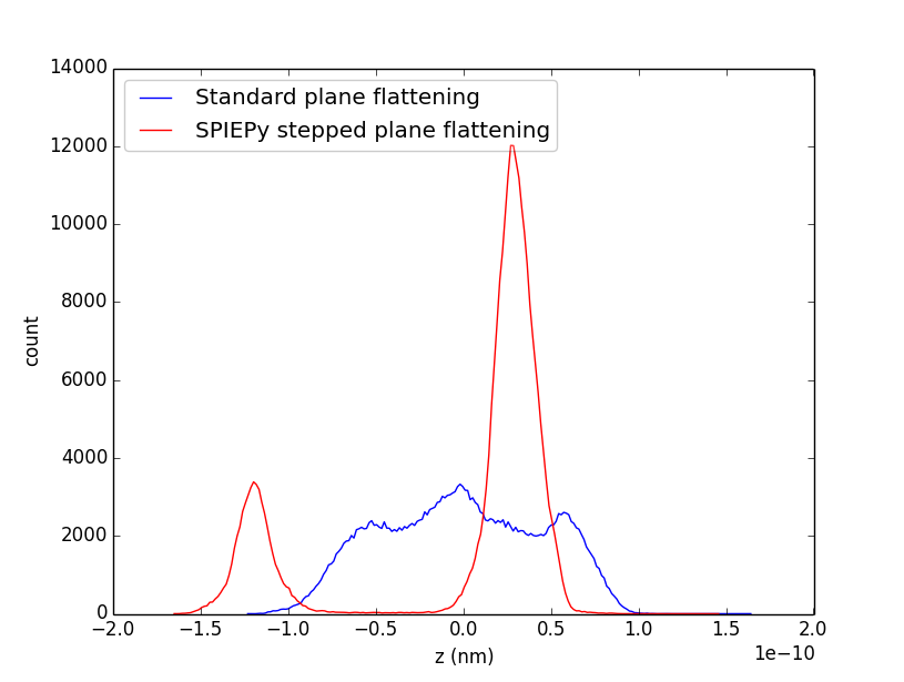
The two terraces are clearly separated!