Flattening Images with Surface Contaminations

In this example you learn how to open a demo image, how to display a image with and without a mask and how to flatten an image with surface contaminations. The surface contaminations and troughs in the object layer will be masked. For flattening the following functions are available:

• flatten_by_iterate_mask()
• flatten_by_peaks()
• flatten_poly_xy()
• flatten_xy()

For masking objects other than objects in the layer:

• mask_by_mean()
• mask_by_troughs_and_peaks()

A Singular Flattening by Masking

Open a Python shell session and import the modules spiepy and spiepy.demo, list the available demo images in SPIEPy:

>>> import spiepy, spiepy.demo
>>> demos = spiepy.demo.list_demo_files()
>>> print demos
{0: 'image_with_defects.dat', 1: 'image_with_step_edge.dat', 2: 'image_with_step_edge_and_atoms.dat'}
>>>

Open the demo image image_with_defects.dat and display the image:

>>> im = spiepy.demo.load_demo_file(demos[0])
>>> import matplotlib.pyplot as plt
>>> plt.imshow(im, cmap = spiepy.NANOMAP, origin = 'lower')
<matplotlib.image.AxesImage object at 0x03FD76F0>
>>> plt.show()

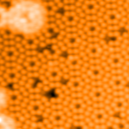
The standard colormap used by most SPM software is the orange colormap NANOMAP. The variable im is the original demo image, you can clearly see that the surface is not level. Now flatten the image with the function flatten_xy():

>>> im_flat, _ = spiepy.flatten_xy(im)

The variable im_flat contains the flattened image, it is the input image minus fitted plane. im is not overwritten, the data will be flattened again later and it is best to avoid cumulative flattening where possible. The flattened image looks like:

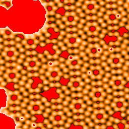
The function mask_by_troughs_and_peaks() is specially engineered for images that has clear atoms, however if the image has not clear atomic contrast it is better to use the function mask_by_mean() to mask the image. Mask out high and low regions and display the flattened image with the mask:

>>> mask, _ = spiepy.mask_by_troughs_and_peaks(im_flat)
>>> palette = spiepy.NANOMAP
>>> palette.set_bad('r', 1.0)
>>> import numpy as np
>>> plot_image = np.ma.array(im_flat, mask = mask)
>>> plt.imshow(plot_image, cmap = palette, origin = 'lower')
<matplotlib.image.AxesImage object at 0x038E1B10>
>>> plt.show()

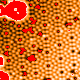
With the mask in the image, you don’t have to look carefully at the image to see that the atoms in the bottom right hand corner appear brighter than those in the top left. This is because of the contamination in the top left corner. Flatten the original image again using the keyword argument mask and the variable mask:

>>> im_flat_m, _ = spiepy.flatten_xy(im, mask)

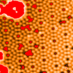
Clearly there is some improvement to uniformity of the atom heights, but the image is not yet truly flat.

Iterative Flattening by Masking

To improve the flattening you can repeat the masking and flattening in a loop. Instead of doing this, SPIEPy has a function which repeats the process until the change in the mask is within an acceptable number of pixels. The function flatten_by_iterate_mask() is very tuneable but with the default values for the keyword arguments it is fast and good. Flatten the original image:

>>> im_flat_fbim, mask, n = spiepy.flatten_by_iterate_mask(im)

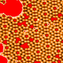
The image is flat to a quite high degree of accuracy, but still some atoms near the centre of the image appear higher than the others. This implies that there might be some image distortion. Often this is removed by a second order polynomial plane flattening, with the masked areas not included. This is possible with the function flatten_poly_xy(), however a more powerful option is available. Now the image is masked you can do a second order polynomial fit through only the peaks of the image which are not in the mask, i.e. the tops of the atoms. Use the function flatten_by_peaks():

>>> im_final, _ = spiepy.flatten_by_peaks(im_flat_fbim, mask)

Continue the shell session and use the final image im_final in the next topic Surface Analysis.