Tutorial

Installation

Installation is easy but requires easy_install and a fortran compiler. I recommend the gfortran compiler. To install scikits.bvp_solver and all its dependencies type “easy_install scikits.bvp_solver” at the command line.

Overview

Solving a boundary value problem using bvp_solver is done in two parts: First, defining the problem, creating a ProblemDefinition object and second, solving it, creating a Solution object which can be called to evaluate the solution at points within the boundaries. At its simplest this works like this:

The ProblemDefinition object is created by supplying its constructor with

• the number of 1st order ODEs in the problem (bvp_solver can only solve a problem with 1st order ODEs, but it is easy to decompose a problem with nth order ODEs into a problem with 1st order ODEs)
• the number of unknown parameters in the problem
• the number of boundary conditions on the left boundary
• an array (or castable) of the two boundary points
• a callback function which evaluates the 1st order ODEs given values for the variables and the unknown parameters
• a callback function which evaluates the difference between the boundary conditions at each boundary and the given values for the variables and the unknown parameters at both boundaries

The solution is generated by calling the solve function and supplying it

• the ProblemDefinition object
• an initial guess for the solution

This process is most easily understood by working though the simple example given below.

A Simple Example

Consider the following boundary value problem:

This boundary value problem describes a counter current heat exchanger; a hot liquid enters a device and exchanges heat across a metal plate with a cold liquid traveling through the device in the opposite direction. Here, T_1 is the temperature of the hot stream, T_2 is the temperature of the cold stream, q is the rate of heat transfer from the hot fluid to the cold fluid, U is the overall heat transfer coefficient and A_hx is the total area of the heat exchanger (in this case we will use 5). In this case the cold stream has twice the thermal mass of the hot stream.

Now let’s write a simple script to solve this boundary value problem (full tutorial example code).

Solving with bvp_solver

The first step is to import bvp_solver and numpy because the callback functions must return numpy arrays:

import scikits.bvp_solver
import numpy

Defining the Problem

The next step is to define the problem by creating a ProblemDefinition object, as we discussed earlier.

First we define the important constants:

T10 = 130
T2Ahx = 70
Ahx = 5
U = 1.0

Then we define the callback function which evaluates the ODEs. The first argument this function receives is the independent variable, in our case A, and the second argument is an array of the values of the dependent variables, in our case, T_1 and T_2. If the boundary value problem includes unknown parameters, then a third argument gets the values of the unknown parameters, but since this problem does not deal with unknown parameters, the function can only have 2 arguments. In this problem we will have the first variable of the dependent variable array represent stream 1 (the hot liquid).

This function must return a numpy array that contains the value of the first derivative of each dependent variable. These must be in the same order as the dependent variable array:

def function(a , T):
    q = (T[0] - T[1]) * U           # calculate the heat transfer from stream 1 to stream 2
    return numpy.array([-q ,        # evaluate dT1/dA
                        q/-2.0])    # evaluate dT2/dA

To finish the problem definition, we define the callback function which evaluates the difference between the actual boundary conditions and the required boundary conditions. The first argument this function receives is an array of the values of the dependent variables (here T_1 and T_2) at the left boundary condition. The second argument this function receives is an array of the values of the dependent variables (here T_1 and T_2) at the right boundary condition.

This function must return two numpy arrays that contains the difference between the actual boundary conditions and the required boundary conditions. The first return array must contain these differences for all boundary conditions on the left, and second return array must contain these differences for all boundary conditions on the right. The sizes of these arrays must add up to the total number of ODEs plus the number of unknown parameters. Both these arrays must be in the same order as the dependent variable arrays (which is the same as in the first function):

def boundary_conditions(Ta,Tb):

    return (numpy.array([Ta[0] - T10]),  #evaluate the difference between the temperature of the hot
                                         #stream on theleft and the required boundary condition
            numpy.array([Tb[1] - T2A]))  #evaluate the difference between the temperature of the cold
                                         #stream on the right and the required boundary condition

Finally we create the ProblemDefinition object, by passing the relevant information and callbacks to its constructor:

problem = scikits.bvp_solver.ProblemDefinition(num_ODE = 2,
                                      num_parameters = 0,
                                      num_left_boundary_conditions = 1,
                                      boundary_points = (0, Ahx),
                                      function = function,
                                      boundary_conditions = boundary_conditions)

Solving

Finally, we solve the boundary value problem by calling the solve function and passing it the ProblemDefinition object and an initial guess for the solution. In this case we will use an array of constants for the guess, simply the average of the temperatures for both streams:

solution = scikits.bvp_solver.solve(problem,
                            solution_guess = ((T10 + T2Ahx)/2.0,
                                              (T10 + T2Ahx)/2.0))

Using the Solution

The solve function returns a Solution object which can be passed an array of points at which to evaluate the solution:

A = numpy.linspace(0,Ahx, 45)
T = solution(A)
print T

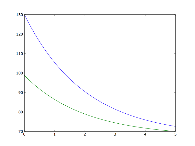
We can plot the solution using pylab with the following code:

import pylab
pylab.plot(A, T[0,:],'-')
pylab.plot(A, T[1,:],'-')
pylab.show()

This gives the following graph. The code for the example in this tutorial is here.