Fitting of Experimental Data¶

Introduction¶

These routines / classes provide a method for fitting of data using mostly least squares methods. There are two main methods here. The pyspec.fit.fit class provides a class for fitting of data. The pyspec.fit.fitdata subroutine serves as a wrapper around the pyspec.fit.fit class. Here the data is taken from the current selected figure. Basically this means that you can fit any set of data which is on the current figure.

The `fit` Class¶

Fitting user supplied data¶

class pyspec.fit.fit(x=None, y=None, e=None, funcs=None, guess=None, quiet=False, optimizer='mpfit', ifix=None, ilimited=None, ilimits=None, xlimits=None, xlimitstype='world', interactive=False, r2min=0.0, debug=0)¶

General class to perform non-linear least squares fitting of data.

This class serves as a wrapper around various fit methods, requiring a standard function to allow for easy fitting of data.

x : ndarray

x data

y : ndarray

y data

e : ndarray

y error

funcs : list

A list of functions to be fitted. These functions should be formed like the standard fitting functions in the pyspec.fitfuncs.

guess : array or string

Array of the initial guess, or string for guess type:

‘auto’ : Auto guess of parameters

quiet : bool

If True then don’t print to the console any results.

ifix : ndarray

An array containing a ‘1’ for fixed parameters

xlimits : ndarray

An (n x 2) array of the limits in x to fit.

xlimitstype : string

Either ‘world’ or ‘index’

optimiser : string :

Optimizer to use for fit: ‘mpfit’, ‘leastsq’, ‘ODR’

interactive : bool

True/False launch interactive fitting mode

r2min : float

If r^2 is less than this value, drop into interactive mode

After a sucsesful fit, the class will contain members for the following.

{fit}.result: result of fit
{fit}.stdev: errors on results (sigma)
{fit}.fit_result: an array of both results and stdev for convinience
{fit}.covar: covarience matrix of result
{fit}.corr: correlation matrix of result
{fit}.r2: R^2 value for fit.

chiSquared(norm=True, dist='poisson')¶

Return the chi-squared value for the fit

Calculate the chi-squared value for the fit. This is defined as: $\chi^2 = \sum_N (x_{d,n} - x_{m,n})$
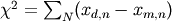
Where d is the data and m is the model. The normalized chi-squared is given by: $\chi^2_{norm} = \chi^2 / M$

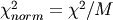
where $M = N - P$ , where P is the number of parameters.

If dist is ‘poisson’ then the data is divided by the model answer. i.e.

$\chi^2_{poisson} = \sum_N {(x_{d,n} - x_{m,i})} / {x_{m,i}}$

norm : bool: If true calculate the normalized chi-squared.
dist : string: The distribution to use, currently only ‘poisson’

chi-squared value

evalfitfunc(nxpts=None, p=None, x=None)¶

Evaluate the fit functions with the fesult of a fit

nxpts : int: Number of x data points if using the range of the input data. If none then the x points of the dataset are used.
p : ndarray: Parameters of function. If None, use current fit result.
x : ndarray: Evaluate fit function at each point defined by the ndarray.

returns f(x) : ndarray

go(interactive=False)¶

Start the fit

interactive : bool: If True, start the fit in interactive mode.

residualSDev()¶: Calculate the sandard deviation of the residuals

run(interactive=False)¶

Start the fit

interactive : bool: If True, start the fit in interactive mode.

textResult()¶: Return a string containing the text results of the fit

Fitting data plotted using matplotlib¶

pyspec.fit.fitdata(funcs, ax=None, showguess=False, *args, **kwargs)¶

Force fitting of a function to graphed data

funcs : list: list of the fit functions
ax : matplotlib axis instance: axis to fit (if none the current axis is used)

All the additional *args and **kwargs are passed onto the fit class (see class pyspec.fit.fit for details).

pyspec.fit.fit instance with result.

Standard Fit Functions¶

pyspec.fitfuncs.constant(x, p, mode='eval')¶

Single constant value

Function:: $f(x) = p_0$

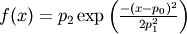
pyspec.fitfuncs.gauss(x, p, mode='eval')¶

Gaussian defined by amplitide

Function:: $f(x) = p_2 \exp\left(\frac{-(x - p_0)^2}{2p_1^2}\right)$

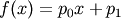
pyspec.fitfuncs.linear(x, p, mode='eval')¶

Linear (strait line)

Function:: $f(x) = p_0 x + p_1$

pyspec.fitfuncs.lor(x, p, mode='eval')¶

Lorentzian defined by amplitude

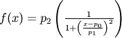
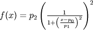
Function:: $f(x) = p_2\left(\frac{1}{1 + \left(\frac{x - p_0}{p_1}\right)^2}\right)$

pyspec.fitfuncs.lor2(x, p, mode='eval')¶

Lorentzian squared defined by amplitude

Function:: $f(x) = p_2\left(\frac{1}{1 + \left(\frac{x - p_0}{p_1}\right)^2}\right)^2$
The HWHM is related to the parameter $\Gamma$ by the relation:: $\kappa = \sqrt{\sqrt{2} - 1}\Gamma$

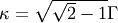
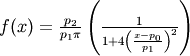
pyspec.fitfuncs.lor2a(x, p, mode='eval')¶: Lorentzian squared function defined by area

pyspec.fitfuncs.lorr(x, p, mode='eval')¶

Lorentzian defined by area

Function:: $f(x) = \frac{p_2}{p_1\pi} \left(\frac{1}{1 + 4\left(\frac{x - p_0}{p_1}\right)^2}\right)$

pyspec.fitfuncs.peakguess(x, y)¶

Guess the “vital statistics” of a peak.

This function guesses the peak’s center width, integral, height and linear background (m, c) from the x and y data passed to it.

pyspec.fitfuncs.power(x, p, mode='eval')¶

Power function

Function:: $f(x) = p_0 p_1^x$

pyspec.fitfuncs.pvoight(x, p, mode='eval')¶

Pseudo Voight function

Function:: :math:’f(x) = ‘

User Defined Functions¶

User defined functions can easily be written. An example of a fit function to provide a linear (straight line) is shown below:

def linear(x, p, mode='eval'):
   if mode == 'eval':
      out = (p[0] * x) + p[1]
   elif mode == 'params':
      out = ['grad','offset']
   elif mode == 'name':
      out = "Linear"
   elif mode == 'guess':
      g = peakguess(x, p)
      out = g[4:6]
   else:
      out = []
   return out

This function is called by the fitting routine each time the function needs to be evaluated. It is also called other times, to gain information about the function. The mode parameter is used to let the function know what is required. The default value of mode should be set to 'eval'. The possible values of mode are discussed below

eval: Evaluate function. Here the function should return $f(x)$ from x and p, where p is the parameters
params: List of parameter names. Here the function should return a list of strings describing the fit parameters. This list should have the same length as the number of fit parameters.
name: Name of the function. Here the function should return a string with a text description of the function.
guess: Parameter guess. Here the function should return a guess of the fit parameters. The function is passed $f(x)$ through the second parameter p. The function should return it’s best guess based on the experimental data, and return those parameters. The peakguess function is provided for convenience which can guess the vital statistics of a peak from the data. This option is not essential but if it is not implemented then the user must provide a numerical guess to the fit class.

Finally, the default response should be to return a null list [].

Fitting of Experimental Data¶

Introduction¶

The `fit` Class¶

Fitting user supplied data¶

Fitting data plotted using matplotlib¶

Standard Fit Functions¶

User Defined Functions¶

Table Of Contents

Previous topic

Next topic

This Page

Navigation

Fitting of Experimental Data¶

Introduction¶

The fit Class¶

Fitting user supplied data¶

Fitting data plotted using matplotlib¶

Standard Fit Functions¶

User Defined Functions¶

Table Of Contents

Previous topic

Next topic

This Page

Quick search

Navigation

The `fit` Class¶