Tutorial 3 - The PyMacLab DSGE instance

Introduction

As already stated in the introduction of the introductory basic tutorial, PyMacLab’s strength or orginal design goal has been that of providing users with a rich and flexible DSGE data structure (also called Class in object-oriented programming speak) which allows them to do lots of interesting things with DSGE models and to treat them as if they were some kind of primitive data type in their own right. While the previous tutorial described some basics as well as the all-important DSGE model file structure and syntax conventions, in this section I am going to stress some of the object-oriented programming features of PyMacLab, in particular the structure of a PyMacLab DSGE model instance or data structure.

Readers with a background in modern programming languages supporting the object-oriented programming (OOP) paradigm will easily relate to concepts in this sections, while for others it may appear more cryptic at first sight. But to convey these concepts to researchers is important, as it stresses many particular advantages of PyMacLab over other programs, and in particular its flexibility, transparency, consistency, persistence and enormous scope for extensibility. All example code fragments provided here assume that you are replicating them within an IPyton interactive session, but they could also be called from a Python program “batch” file.

Understanding the PyMacLab DSGE model class and its instances

PyMacLab has been written in the Python programming language which supports object-oriented programming. This means, that more than 80% of PyMacLab’s code is devoted to the definition of data fields and methods of the DSGE_model Class, which forms the basis for all DSGE models users can load, spawn or instantiate and interact with once they have imported they PyMacLab library into their programs. As already explained elsewhere, the basis of all DSGE model instances is the DSGE model’s model text file in which it is defined in terms of its specific characteristics, such as its parameters and first-order conditions of optimality. We recall that this process of loading or instantiating a DSGE model worked as follows:

# Import the pymaclab module into its namespace, also import os module
In [1]: import pymaclab as pm
In [2]: from pymaclab.modfiles import models

# Instantiate a new DSGE model instance like so
In [4]: rbc1 = pm.newMOD(models.stable.rbc1)

After executing these lines of code in an interactive environment such as that provided by IPython, which emulates well the feel and behaviour of the Matlab interactive environment, the DSGE instance or data object going by the name of rbc1 now exists in the namespace of the running program and can be put to further use. But before looking at these various ways possible to make effective use of this DSGE model instance, let’s first trace the various steps the programs goes through when a DSGE model get instantiated. So what happens internally when the above last line in the code fragment is called:

1. The empty shell DSGE model instance gets instantiated
2. The DSGE model instance reads the model file provided to it and any other arguments and saves them by attaching them to itself.
3. Instantiation Step 1: The files get read in and a method defined on the instance simply splits the file into its individual sections and saves these raw sections by attaching them to itself.
4. Instantiation Step 2: A parser method is called which disaggregates the raw information provided in each section of the model file and begins to extract meaningful information from it, each time saving this information by attaching it to itself as data fields. Also, the DSGE model instance is prepared and set up in order to attempt to solve for the steady state of it manually at the command line, instead of doing it automatically. If you want the model instance to do ONLY this next step and stop there for you to explore further interactively, you must call the command with and extra argument like this:

# Import the pymaclab module into its namespace, also import os module
In [1]: import pymaclab as pm
In [2]: from pymaclab.modfiles import models

# Instantiate a new DSGE model instance like so, but adding initlev=0 as extra argument
In [3]: rbc1 = pm.newMOD(models.stable.rbc1,initlev=0)

5. Instantiation Step 3: The information is used in order to attempt to compute the numerical steady-state of the model. If you want the model instance to do ONLY this next step and stop there for you to explore further interactively, you must call the command with and extra argument like this:

# Import the pymaclab module into its namespace, also import os module
In [1]: import pymaclab as pm
In [2]: from pymaclab.modfiles import models

# Instantiate a new DSGE model instance like so, but adding initlev=1 as extra argument
In [3]: rbc1 = pm.newMOD(models.stable.rbc1,initlev=1)

6. Instantiation Step 4: If the steady state was computed successfully then the model’s analytical and numerical Jacobian and Hessian are computed. Finally a preferred dynamic solution method is called which solves the model for its policy function and other laws of motion.

To give users a choice of “solution depths” at DSGE object instantiation time is important and useful, especially in the initial experimentation phase during which the DSGE model file gets populated. That way researchers can first carefully solve one part of the problem (i.e. looking for the steady state) and indeed choose to do so manually on the IPython interactive command shell, allowing them to immediately inspect any errors.

Instantiation options for DSGE model instances

There are a couple of instance invocation or instantiation arguments one should be aware of. At the time of writing these lines there are in total 5 other arguments (besides the DSGE model template file path) which can be passed to the pymaclab.newMOD function out of which 1 is currently not (yet) supported and not advisable to employ. The other 4 options determine the initiation level of the DSGE model (i.e. how far it should be solved if at all), whether diagnosis messages should be printed to screen during instantiation, how many CPU cores to employ when building the Jacobian and Hessian of the model, and finally whether the expensive-to-compute Hessian should be computed at all. Remember that the last option is useful as many researchers often - at least initially - want to explore the solution to their model to a first order of approximation before taking things further. So here are the options again in summary with their default values:

Option with default value	Description
pm.newMOD(mpath,initlev=2)	Initlev=0 only parses and prepares for manual steady state calculation
	Initlev=1 does initlev=0 and attempts to solve for the model’s steady state automatically
	Initlev=2 does initlev=0, initlev=1 and generates Jacobian and Hessian and solves model dynamically
pm.newMOD(mpath,mesg=False)	Prints very useful runtime instantiation messages to the screen for users to follow progress
pm.newMOD(mpath,ncpus=1)	CPU cores to be used in expensive computation of model’s derivatives, ‘auto’ for auto-detection
pm.newMOD(mpath,mk_hessian=True)	Should Hessian be computed at all, as is expensive?
pm.newMOD(mpath,use_focs=False)	Should only the model’s FOCs be used to computed the steady state? Accepts Python list or tuple
pm.newMOD(mpath,ssidic=None)	Use in conjunction with previous argument to specify initial starting values as Python dictionary
pm.newMOD(mpath,sstate=None)	Specify steady state values as Python dictionary and supply here. No SS computation in instance

Needless to say, all of the options can be and usually are called in combination, they are only shown separately here for sake of expositional clarity. Medium-sized to large-sized models can take considerable time to compute the Jacobian alone, let alone the Hessian. On the other hand passing more (real as opposed to virtual) CPU cores to the instantiation process can significantly cut down computation time. In this case, the FOCs nonlinear equations are distributed to individual cores for analytical differentiation as opposed to doing this serially on one CPU core.

Working with DSGE model instances

The most useful feature is to call the model with the option initlev=0, because this will allow you more control over the steady-state computation of the model by permitting a closer interactive inspection of the DSGE model instance as created thus far. Let’s demonstrate this here:

# Import the pymaclab module into its namespace, also import os module
In [1]: import pymaclab as pm
In [2]: from pymaclab.modfiles import models

# Instantiate a new DSGE model instance like so, but adding initlev=0 as extra argument
In [3]: rbc1 = pm.newMOD(models.stable.rbc1,initlev=0)

# This datafield contains the original nonlinear system expressed as g(x)=0
In [4]: rbc1.sssolvers.fsolve.ssm
['z_bar*k_bar**(rho)-delta*k_bar-c_bar',
 'rho*z_bar*k_bar**(rho-1)+(1-delta)-R_bar',
 '(betta*R_bar)-1',
 'z_bar*k_bar**(rho)-y_bar']

# This datafield contains the initial values supplied to the rootfinder algorithm
In [5]: rbc1.sssolvers.fsolve.ssi
{'betta': 1.0, 'c_bar': 1.0, 'k_bar': 1.0, 'y_bar': 1.0}

# Instead of letting the model during instantiation solve the model all the way through,
# we can solve for the steady state by hand, manually
In [6]: rbc1.sssolvers.fsolve.solve()

# And then inspect the solution and some message returned by the rootfinder
In [6]: rbc1.sssolvers.fsolve.fsout
{'betta': 0.9900990099009901,
 'c_bar': 2.7560505909330626,
 'k_bar': 38.1607004898424,
 'y_bar': 3.7100681031791227}

In [7]: rbc1.sssolvers.fsolve.mesg
'The solution has converged.'

Another useful lesson to take away from this example is that a DSGE model instance is like a many-branch tree structure, just like the Windows File Explorer so many people are familiar with, where individual “nodes” represent either data fields or methods (function calls) which equip the model instance with some functionality. This kind of approach of structuring and programming a solution to the problem of designing a program which handles the solution-finding of DSGE models offers enormous scope for experimentation and extensibility. After a DSGE model has been instantiated without passing the initlev argument, you can inspect this structure like so:

# Import the pymaclab module into its namespace, also import os module
In [1]: import pymaclab as pm
In [2]: from pymaclab.modfiles import models

# Instantiate a new DSGE model instance like so
In [3]: rbc1 = pm.newMOD(models.stable.rbc1)

# Inspect the data fields and methods of the DSGE model instance
In [4]: dir(rbc1)
['__class__',
 '__delattr__',
 '__dict__',
 '__doc__',
 '__format__',
 '__getattribute__',
 '__hash__',
 '__init__',
 '__module__',
 '__new__',
 '__reduce__',
 '__reduce_ex__',
 '__repr__',
 '__setattr__',
 '__sizeof__',
 '__str__',
 '__subclasshook__',
 '__weakref__',
 '_initlev',
 'audic',
 'author',
 'ccv',
 'dbase',
 'deltex',
 'getdata',
 'info',
 'init2',
 'manss_sys',
 'mkeigv',
 'mkjahe',
 'mkjahen',
 'mkjahenmat',
 'mkjahepp',
 'mkjaheppn',
 'mod_name',
 'modfile',
 'nall',
 'ncon',
 'nendo',
 'nexo',
 'nlsubs',
 'nlsubs_list',
 'nlsubs_raw1',
 'nlsubs_raw2',
 'nother',
 'nstat',
 'numssdic',
 'paramdic',
 'pdf',
 'setauthor',
 'ssidic',
 'sssolvers',
 'sstate',
 'ssys_list',
 'subs_vars',
 'switches',
 'texed',
 'txted',
 'txtpars',
 'updf',
 'updm',
 'vardic',
 'vreg']

As you can see, the attributes exposed at the root of the instance are plenty and can be acccessed in the usual way:

# Import the pymaclab module into its namespace, also import os module
In [1]: import pymaclab as pm
In [2]: from pymaclab.modfiles import models

# Instantiate a new DSGE model instance like so
In [3]: rbc1 = pm.newMOD(models.stable.rbc1)

# Access one of the model's fields
In [4]: rbc1.ssys_list
['z_bar*k_bar**(rho)-delta*k_bar-c_bar',
'rho*z_bar*k_bar**(rho-1)+(1-delta)-R_bar',
'(betta*R_bar)-1',
'z_bar*k_bar**(rho)-y_bar']

So one can observe that the data field rbc1.ssys_list simply summarizes the system of nonlinear equations which has been described in the relevant section of the DSGE model file. Now you know how to explore the DSGE model instance and understand its general structure, and we conclude this short tutorial by inviting you to do so. Don’t forget that some nodes at the root possess further sub-nodes, as was the case when cascading down the rbc1.sssolvers branch. To help your search, the only other node with many more sub-nodes is the rbc1.modsolvers branch, which we will explore more in the next section to this tutorial series.

DSGE modelling made intuitive

Before concluding this tutorial, we will demonstrate how PyMacLab’s DSGE data structure (or instance) approach allows researchers to implement ideas very intuitively, such as for instance “looping” over a DSGE model instance in order to explore how incremental changes to the parameter space alter the steady state of the model. Leaving our usual interactive IPyton shell, consider the following Python program file:

# Import the pymaclab module into its namespace
# Also import Numpy for array handling and Matplotlib for plotting
import pymaclab as pm
from pymaclab.modfiles import models
import numpy as np
from matplotlib import pyplot as plt

# Instantiate a new DSGE model instance like so
rbc1 = pm.newMOD(models.stable.rbc1)

# Create an array representing a finely-spaced range of possible impatience values
# Then convert to corresponding steady state gross real interest rate values
betarr = np.arange(0.8,0.99,0.001)
betarr = 1.0/betarr

# Loop over the RBC DSGE model, each time re-computing for new R_bar
ss_capital = []
for betar in betarr:
    rbc1.updaters.paramdic['R_bar'] = betar # assign new R_bar to model
    rbc1.sssolvers.fsolve.solve() # re-compute steady stae
    ss_capital.append(rbc1.sssolvers.fsolve.fsout['k_bar']) # fetch and store k_bar

# Create a nice figure
fig1 = plt.figure()
plt.grid()
plt.title('Plot of steady state physical capital against R\_bar')
plt.xlabel(r'Steady state gross real interest rate')
plt.ylabel(r'Steady State of physical capital')
plt.plot(betarr,ss_capital,'k-')
plt.show()

Anybody who has done some DSGE modelling in the past will easily be able to intuitively grasp the purpose of the above code snippet. All we are doing here is to loop over the same RBC model, each time feeding it with a slightly different steady state groos real interest rate value and re-computing the steady state of the model. This gives rise to the following nice plot exhibting the steady state relationship between the interest rate and the level of physical capital prevailing in steady state:

(Source code, png, hires.png, pdf)

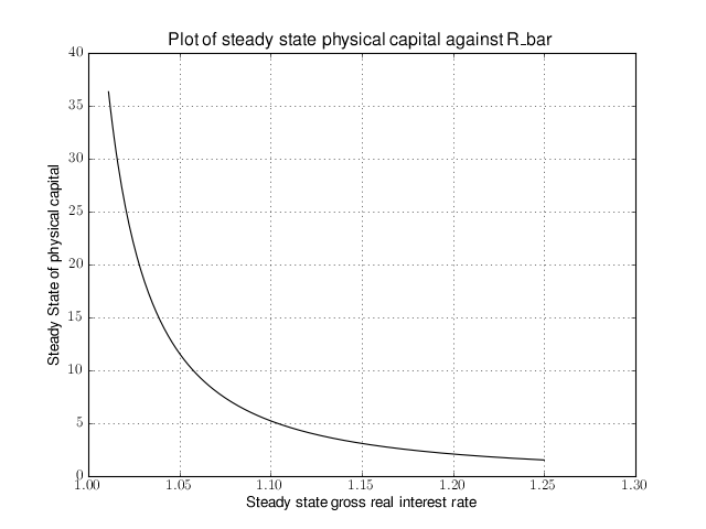
That was nice and simple, wasn’t it? So with the power and flexibility of PyMacLab DSGE model instances we can relatively painlessly explore simple questions such as how differing deep parameter specifications for the impatience factor can affect the steady state level of physical capital. And indeed, as intuition would suggest, less patient consumers are less thrifty and more spend-thrifty thus causing a lower steady state level of physical capital in the economy. This last example also serves to make another important point. PyMacLab is not a program such as Dynare, but instead an add-in library for Python prividing an advanced DSGE model data structure in form of a DSGE model class which can be used in conjunction with any other library available in Python.