A simple real business cycle model without a labour-leisure choice
Introduction
This model was popularized by these people.
Model Setup
Households
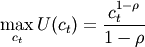
In our simple RBC model involving no labour-leisure choice, our housholds’ momentary utility function depends only on consumption in period t. Also, households are assumed to pick levels of consumption which maximize this function over the their entire (typically infinite) lifetimes.
(1)
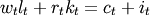
The household’s budget contstraint can be expressed in a number of different ways, all of which are equivalent to each other:
(2)
which is the most simple method of stating the houshold’s budget constraint, simply implying that output has to be exhausted on consumption investment.
(3)
The second method more explicitly spells out how output is produced via a CRS Cobb-Douglas production function as well as how investment is related to the perpetual inventory model.
(4)
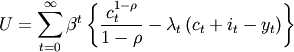
Finally, the last method describes how total income is exhausted through expenditure on consumption and investment. Since the household optimizes over her its lifetime subject to the budget constraint, the complete problem would be expressible as:
(5)
Firms
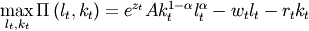
Firms in this model are assumed to be profit-maximizing and to be renting factors of production in competitive input factor markets. This means
that for one of labour they pay the competitive wage rate  and for one unit of physical capital they pay the real
interest rate
and for one unit of physical capital they pay the real
interest rate  . Therefore:
(6)
Strictly speaking we could also spell out the firm’s problem as one which is solved over infinitely many periods. However, since the firm faces an identical problem in each time period, there is no inter-temporality involved here, so we can just focus on the within-period problem which would be optimal for all periods.
First-Order Conditions of Optimality
The first-order conditions of optimality are simply obtained by setting up both the household’s and the firm’s contrained optimisation problems and taking first derivatives.
Households
(7)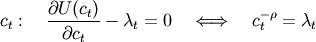
where  is simply equal to the shadow price of one unit of wealth. This condition simply states that at an optimum
the marginal utility of consumption has to equal the marginal value in utility terms of one extra unit of wealth. Households also have to decide
on how much of their wealth to invest in the physical capital storage technology
is simply equal to the shadow price of one unit of wealth. This condition simply states that at an optimum
the marginal utility of consumption has to equal the marginal value in utility terms of one extra unit of wealth. Households also have to decide
on how much of their wealth to invest in the physical capital storage technology  , formally a decision of how much to save:
(8)
When using the FOC for consumption as well as being more explicit about the real rate of return, we can also write the above as [1] :
(9)
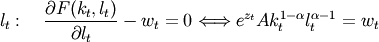
Firms
Firms have to choose optimal quantities of labour and physical capital in order to produce their output and maximize their profits. This leads to the first-order conditions of optimality:
(10)
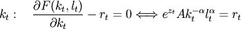
and for physical capital:
(11)
any solution needs to respect the original budget constraint:
(12)
Footnotes
| [1] | Journal articles and text book treatments often use different notations for next-period capital. Sometimes it is written as
to stress the fact that next-period  capital is determined in this period capital is determined in this period  , while at other times
it is written as , while at other times
it is written as  to stress the fact that this will be the amount of capital available next period after it
was determined in this period. to stress the fact that this will be the amount of capital available next period after it
was determined in this period. |