Proximal total-variation operators
proxTV is a toolbox implementing blazing fast implementations of Total Variation proximity operators.
The library provides efficient solvers for the following Total Variation proximity problems:
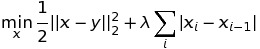
Standard (l1) Total Variation on a 1-dimensional signal
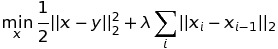
Quadratic (l2) Total Variation on a 1-dimensional signal
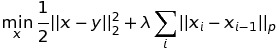
lp-norm Total Variation on a 1-dimensional signal
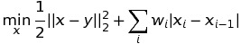
Weighted Total Variation on a 1-dimensional signal
Anisotropic Total Variation on a 2-dimensional signal
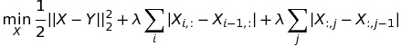
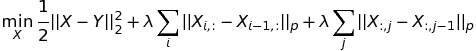
lp-norm Anisotropic Total Variation on a 2-dimensional signal
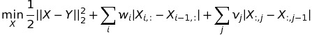
Weighted Anisotropic Total Variation on a 2-dimensional signal
Anisotropic Total Variation on a 3-dimensional signal

Generalized N-dimensional Anisotropic Total Variation
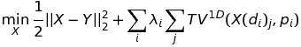
(with X(di) every possible 1-dimensional slice of X following dimension di)
As a general rule the functions in this package have the form tv<a>[w]_<b>d, where:
- <a> : 1, 2 or p, if the norm is \(\ell_1\), \(\ell_2\) or the general \(\ell_p\)
- [w] : if present, the methods accepts a weighted norm.
- <b> : 1 or 2, if the expected signals is 1- or 2-dimensional.
The only expection is the function tvgen that solves generalized Total Variation problems, recommended only to advanced users.
As the underlying library uses FORTRAN-style matrices (column-order), the given matrices will be converted to this format if necessary.
If you find this toolbox useful please reference the following papers:
- Fast Newton-type Methods for Total Variation Regularization. Alvaro Barbero, Suvrit Sra. ICML 2011 proceedings.
- Modular proximal optimization for multidimensional total-variation regularization. Alvaro Barbero, Suvrit Sra. http://arxiv.org/abs/1411.0589
Function reference
One dimensional total variation problems
- prox_tv._prox_tv.tv1_1d(x, w, sigma=0.05, method='tautstring')
1D proximal operator for \(\ell_1\).
Specifically, this optimizes the following program:
\[\mathrm{min}_y \frac{1}{2} \|x-y\|^2 + w \sum_i |y_i - y_{i+1}|.\]Parameters: - y (numpy array) – The signal we are approximating.
- w (float) – The non-negative weight in the optimization problem.
- method (str) –
The algorithm to be used, one of:
- 'tautstring'
- 'pn' - projected Newton.
- 'condat' - Condat’s segment construction method.
- 'dp' - Johnson’s dynamic programming algorithm.
- sigma (float) – Tolerance for sufficient descent (used only if method='pn').
Returns: The solution of the optimization problem.
Return type: numpy array
- prox_tv._prox_tv.tv1w_1d(x, w, method='tautstring', sigma=0.05)
Weighted 1D proximal operator for \(\ell_1\).
Specifically, this optimizes the following program:
\[\mathrm{min}_y \frac{1}{2} \|x-y\|^2 + \sum_i w_i |y_i - y_{i+1}|.\]Parameters: - y (numpy array) – The signal we are approximating.
- w (numpy array) – The non-negative weights in the optimization problem.
- method (str) – Either 'tautstring' or 'pn' (projected Newton).
- sigma (float) – Tolerance for sufficient descent (used only if method='pn').
Returns: The solution of the optimization problem.
Return type: numpy array
- prox_tv._prox_tv.tv2_1d(x, w, method='mspg')
1D proximal operator for \(\ell_2\).
Specifically, this optimizes the following program:
\[\mathrm{min}_y \frac{1}{2} \|x-y\|^2 + w \sum_i (y_i - y_{i+1})^2.\]Parameters: - y (numpy array) – The signal we are approximating.
- w (float) – The non-negative weight in the optimization problem.
- method (str) –
One of the following:
- 'ms' - More-Sorenson.
- 'pg' - Projected gradient.
- 'mspg' - More-Sorenson + projected gradient.
Returns: The solution of the optimization problem.
Return type: numpy array
- prox_tv._prox_tv.tvp_1d(x, w, p, method='gpfw', max_iters=0)
1D proximal operator for any \(\ell_p\) norm.
Specifically, this optimizes the following program:
\[\mathrm{min}_y \frac{1}{2} \|x-y\|^2 + w \|y_i - y_{i+1}\|_p.\]Parameters: - y (numpy array) – The signal we are approximating.
- w (float) – The non-negative weight in the optimization problem.
- method (str) –
The method to be used, one of the following:
- 'gp' - gradient projection
- 'fw' - Frank-Wolfe
- 'gpfw' - hybrid gradient projection + Frank-Wolfe
Returns: The solution of the optimization problem.
Return type: numpy array
Two dimensional total variation problems
- prox_tv._prox_tv.tv1_2d(x, w, n_threads=1, max_iters=0, method='dr')
2D proximal oprator for \(\ell_1\).
Specifically, this optimizes the following program:
\[\mathrm{min}_y \frac{1}{2} \|x-y\|^2 + w \sum_{i,j} (|y_{i, j} - y_{i, j+1}| + |y_{i,j} - y_{i+1,j}|).\]Parameters: - y (numpy array) – The signal we are approximating.
- w (float) – The non-negative weight in the optimization problem.
- str (method) –
One of the following:
- 'dr' - Douglas Rachford splitting.
- 'pd' - Proximal Dykstra splitting.
- 'yang' - Yang’s algorithm.
- 'condat' - Condat’s gradient.
- 'chambolle-pock' - Chambolle-Pock’s gradient.
- n_threads (int) – Number of threads, used only for Proximal Dykstra and Douglas-Rachford.
Returns: The solution of the optimization problem.
Return type: numpy array
- prox_tv._prox_tv.tv1w_2d(x, w_col, w_row, max_iters=0, n_threads=1)
2D weighted proximal operator for \(\ell_1\) using DR splitting.
Specifically, this optimizes the following program:
\[\mathrm{min}_y \frac{1}{2} \|x-y\|^2 + \sum_{i,j} w^c_{i, j} |y_{i,j} - y_{i, j+1}| + w^r_{i, j} |y_{i,j}-y_{i+1,j}|.\]Parameters: - y (numpy array) – The MxN matrix we are approximating.
- w_col (numpy array) – The (M-1) x N matrix of column weights \(w^c\).
- w_row (numpy array) – The M x (N-1) matrix of row weights \(w^r\).
Returns: The MxN solution of the optimization problem.
Return type: numpy array
- prox_tv._prox_tv.tvp_2d(x, w_col, w_row, p_col, p_row, n_threads=1, max_iters=0)
2D proximal operator for any \(\ell_p\) norm.
Specifically, this optimizes the following program:
\[\mathrm{min}_y \frac{1}{2}\|x-y\|^2 + w^r \|D_\mathrm{row}(y)\|_{p_1} + w^c \|D_\mathrm{col}(y) \|_{p_2},\]where \(\mathrm D_{row}\) and \(\mathrm D_{col}\) take the differences accross rows and columns respectively.
Parameters: - y (numpy array) – The matrix signal we are approximating.
- p_col (float) – Column norm.
- p_row (float) – Row norm.
- w_col (float) – Column penalty.
- w_row (float) – Row penalty.
Returns: The solution of the optimization problem.
Return type: numpy array
Generalized total variation problems
- prox_tv._prox_tv.tvgen(x, ws, ds, ps, n_threads=1, max_iters=0)
General TV proximal operator for multidimensional signals
Specifically, this optimizes the following program:
\[\min_X \frac{1}{2} ||X-Y||^2_2 + \sum_i w_i \sum_j TV^{1D}(X(d_i)_j,p_i)\]where \(X(d_i)_j\) every possible 1-dimensional fiber of X following the dimension d_i, and \(TV^{1D}(z,p)\) the 1-dimensional \(\ell_p\)-norm total variation over the given fiber \(z\). The user can specify the number \(i\) of penalty terms.
Parameters: - y (numpy array) – The matrix signal we are approximating.
- ws (list) – Weights to apply in each penalty term.
- ds (list) – Dimensions over which to apply each penalty term. Must be of equal length to ws.
- ps (list) – Norms to apply in each penalty term. Must be of equal length to ws.
- n_threads (int) – number of threads to use in the computation
- max_iters (int) – maximum number of iterations to run the solver.
Returns: The solution of the optimization problem.
Return type: numpy array
Examples
1D examples
Filter 1D signal using TV-L1 norm:
tv1_1d(x, w)
Filter 1D signal using weighted TV-L1 norm (for x vector of length N, weights vector of length N-1):
tv1w_1d(x, weights)
Filter 1D signal using TV-L2 norm:
tv2_1d(x, w)
Filter 1D signal using both TV-L1 and TV-L2 norms:
tvgen(X, [w1, w2], [1, 1], [1, 2])
2D examples
Filter 2D signal using TV-L1 norm:
tv1_2d(X, w)
or:
tvgen(X, [w, w], [1, 2], [1, 1])
Filter 2D signal using TV-L2 norm:
tvp_2d(X, w)
or:
tvgen(X, [w, w], [1, 2], [2, 2])
Filter 2D signal using 4 parallel threads:
tv1_2d(X, w, n_threads=4)
or:
tvgen(X, [w, w], [1, 2], [1, 1], n_threads=4)
Filter 2D signal using TV-L1 norm for the rows, TV-L2 for the columns, and different penalties:
tvgen(X, [wRows, wCols], [1, 2], [1, 2])
Filter 2D signal using both TV-L1 and TV-L2 norms:
tvgen(X, [w1, w1, w2, w2], [1, 2, 1, 2], [1, 1, 2, 2])
Filter 2D signal using weighted TV-L1 norm (for X image of size MxN, W1 weights of size (M-1)xN, W2 weights of size Mx(N-1)):
tv1w_2d(X, W1, W2)
3D examples
Filter 3D signal using TV-L1 norm:
tvgen(X, [w, w, w], [1, 2, 3], [1, 1, 1])
Filter 3D signal using TV-L2 norm, not penalizing over the second dimension:
tvgen(X , [w, w], [1, 3], [2, 2])