oemof.solph package¶

Submodules¶

oemof.solph.linear_constraints module¶

The linear_contraints module contains the pyomo constraints wrapped in functions. These functions are used by the ‘_assembler- methods of the OptimizationModel()-class.

The module frequently uses the dictionaries I and O for the construction of constraints. I and O contain all components’ uids as dictionary keys and the relevant input input/output uids as dictionary items.

Illustrative Example:

Consider the following example of a chp-powerplant modeled with 4 entities (3 busses, 1 component) and their unique ids being stored in a list called uids:
>>> uids = ['bus_el', 'bus_th', 'bus_coal','pp_coal']
>>> I = {'pp_coal': 'bus_coal'}
>>> O = {'pp_coal': ['bus_el', 'bus_th']}
>>> print(I['pp_coal'])
'bus_el'

In mathematical notation I, O can be seen as indexed index sets The elements of the sets are the uids of all components (index: e). The the inputs/outputs uids are the elements of the accessed set by the component index e. Generally the index e is the index for the uids-sets containing the uids of objects for which the constraints are build. For all mathematical constraints the following definitions hold:

Inputs: $I(e) = \text{Input-uids of entity } e \in E$

Outputs: $O(e) = \text{All output-uids of entity } e \in E$

As components may have multiple outputs they are grouped in subsets. The order is given by the order of outputs inside the attribute outputs of the entitiy.

$O_1(e) = \text{First output-uids of entity } e \in E$

$O_2(e) = \text{Second output-uids of entity } e \in E$

Entities: $E = \{uids\},$

Timesteps: $t \in T = \{timesteps\}$

Simon Hilpert (simon.hilpert@fh-flensburg.de)

oemof.solph.linear_constraints.add_bus_balance(model, block=None)[source]¶

Adds constraint for the input-ouput balance of bus objects.

The mathematical formulation for the balance is as follows:

$\sum_{i \in I(e)} W(i, e, t) = \sum_{o \in O(e)} W(e, o, t), \qquad \forall e, \forall t$

With $e \in E$ and $E$ beeing the set of unique ids for all entities grouped inside the attribute block.objs.

$O(e)$ beeing the set of all outputs of entitiy (bus) $e$ .

$I(e)$ beeing the set of all inputs of entitiy (bus) $e$ .

Parameters:	model (OptimizationModel() instance) – block (SimpleBlock()) –

oemof.solph.linear_constraints.add_dispatch_source(model, block)[source]¶

Creates dispatchable source bounds/constraints.

First the maximum value for the output of the source will be set. Then a constraint is defined that determines the dispatch of the source. This dispatch can be used in the objective function to add cost for dispatch of sources.

The mathemathical formulation of the constraint is as follows:

$CURTAIL(e,t) = val_{norm}(e,t) \cdot out_{max}(e) - W(e,O_1(e),t), \qquad \forall e, \forall t$

With $e \in E$ and $E$ beeing the set of unique ids for all entities grouped in the attribute block.objs.

$O_1(e)$ beeing the set of all first outputs of entitiy (component) $e$ .

Parameters:	model (OptimizationModel() instance) – An object to be solved containing all Variables, Constraints, Data. block (SimpleBlock()) –

oemof.solph.linear_constraints.add_eta_total_chp_relation(model, block)[source]¶

Adds constraints for input-(output1,output2) relation as simple function for all objects in block.objs.

The mathematical formulation of the input-output relation of a simple transformer is as follows:

$W(I(e), e, t) \cdot \eta_{total}(e) = W(e, O_1(e), t) + W(e, O_2(e), t), \qquad \forall e, \forall t$

With $e \in E$ and $E$ beeing the set of unique ids for all entities grouped inside the attribute block.objs.

$O_1(e)$ beeing the set of all first outputs of entitiy (component) $e$ .

$O_2(e)$ beeing the set of all first outputs of entitiy (component) $e$ .

$I(e)$ beeing the set of all inputs of entitiy (component) $e$ .

Parameters:	model (OptimizationModel() instance) – An object to be solved containing all Variables, Constraints, Data. block (SimpleBlock()) –

oemof.solph.linear_constraints.add_fixed_source(model, block)[source]¶

Sets fixed source bounds and constraints for all objects in block.objs

The mathematical formulation is as follows:

$W(e,O(e),t) = val_{norm}(e,t) \cdot out_{max}(e), \qquad \forall e, \forall t$

For investment for component:

$W(e, O_1(e), t) \leq (out_{max}(e) + ADDOUT(e) \cdot val_{norm}(e,t), \qquad \forall e, \forall t$

$ADDOUT(e) \leq addout_{max}(e), \qquad \forall e$

With $e \in E$ and $E$ beeing the set of unique ids for all entities grouped inside the attribute block.objs.

$O_1(e)$ beeing the set of all outputs of entitiy (component) $e$ . ———- model : OptimizationModel() instance

An object to be solved containing all Variables, Constraints, Data.

block : SimpleBlock()

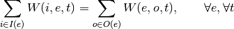
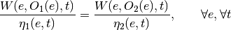
oemof.solph.linear_constraints.add_global_output_limit(model, block=None)[source]¶

Adds constraints to set limit for variables as sum over the total timehorizon for all objects in block.objs

The mathematical formulation is as follows:

$\sum_{t \in T} \sum_{o \in O(e)} W(e, o, t) \leq sumlimit_{out}(e), \qquad \forall e \in E$

With $e \in E$ and $E$ beeing the set of unique ids for all entities grouped in the attribute block.objs.

$O(e)$ beeing the set of all outputs of entitiy $e$ .

Parameters:	model (OptimizationModel() instance) – An object to be solved containing all Variables, Constraints, Data. block (SimpleBlock()) –

oemof.solph.linear_constraints.add_output_gradient_calc(model, block, grad_direc='both')[source]¶

Add constraint to calculate the gradient between two timesteps (positive and negative)

The mathematical formulation for constraints are as follows:

Positive gradient:

$W(e,O_1(e),t) - W(e,O(e),t-1) \leq GRADPOS(e,t) \qquad \forall e, \forall t / t=1$

$GRADPOS(e,t) \leq gradpos_{max}(e), \qquad \forall e, \forall t$

Negative gradient:

$W(e,O_1(e),t-1) - W(e,O(e),t) \leq GRADNEG(e,t) \qquad \forall e, \forall t / t=1$

$GRADNEG(e,t) \leq gradneg_{max}(e), \qquad \forall e, \forall t$

With $e \in E$ and $E$ beeing the set of unique ids for all entities grouped inside the attribute block.objs.

$O_1(e)$ beeing the set of all first outputs of entitiy (component) $e$ .

Parameters:	model (OptimizationModel() instance) – An object to be solved containing all Variables, Constraints, Data. block (SimpleBlock()) – grad_direc (string) – string defining the direction of the gradient constraint. (‘positive’, negative’, ‘both’)

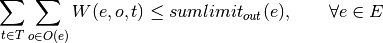
oemof.solph.linear_constraints.add_simple_chp_relation(model, block)[source]¶

Adds constraint for output-output relation for all simple combined heat an power units in block.objs.

The mathematical formulation for the constraint is as follows:

$\frac{W(e,O_1(e),t)}{\eta_1(e,t)} = \frac{W(e, O_2(e), t)}{\eta_2(e,t)}, \qquad \forall e, \forall t$

With $e \in E$ and $E$ beeing the set of unique ids for all entities grouped inside the attribute block.objs.

$O_1(e)$ beeing the set of all first outputs of entitiy (component) $e$ .

$O_2(e)$ beeing the set of all second outputs of entitiy (component) $e$ .

$I(e)$ beeing the set of all inputs of entitiy (component) $e$ .

Parameters:	model (OptimizationModel() instance) – An object to be solved containing all Variables, Constraints, Data. block (SimpleBlock()) –

oemof.solph.linear_constraints.add_simple_extraction_chp_relation(model, block)[source]¶

Adds constraints for power to heat relation and equivalent output for a simple extraction combined heat an power units. The constraints represent the PQ-region of the extraction unit and are set for all objects in block.objs

The mathematical formulation is as follows:

For Power/Heat ratio:

$W(e,O_1(e),t) = W(e, O_2(e), t) \cdot \sigma(e), \qquad \forall e, \forall t$

$\sigma(e) = \text{Power to heat ratio of entity } e$

For euivalent power:

$W(I(e),e,t) = \frac{(W(e,O_1(e),t) + \beta(e) \cdot W(e, O_2(e), t))}{\eta_1(e)}$

$\beta(e) = \text{Power loss index of entity } e$

With $e \in E$ and $E$ beeing the set of unique ids for all entities grouped inside the attribute block.objs.

$O_1(e)$ beeing the set of all first outputs of entitiy (component) $e$ .

$O_2(e)$ beeing the set of all second outputs of entitiy (component) $e$ .

$I(e)$ beeing the set of all inputs of entitiy (component) $e$ .

Parameters:	model (OptimizationModel() instance) – An object to be solved containing all Variables, Constraints, Data. block (SimpleBlock()) –

oemof.solph.linear_constraints.add_simple_io_relation(model, block, idx=0)[source]¶

Adds constraints for input-output relation as simple function for all objects in block.objs.

The mathematical formulation of the input-output relation of a simple transformer is as follows:

$W(I(e), e, t) \cdot \eta(e) = W(e, O_1(e), t), \qquad \forall e, \forall t$

With $e \in E$ and $E$ beeing the set of unique ids for all entities grouped inside the attribute block.objs.

$O_1(e)$ beeing the set of all first outputs of entitiy (component) $e$ .

$I(e)$ beeing the set of all inputs of entitiy (component) $e$ .

Parameters:	model (OptimizationModel() instance) – An object to be solved containing all Variables, Constraints, Data. block (SimpleBlock()) – idx (integer) – Index to choose which output to select (from list of Outputs: O[e][idx])

oemof.solph.linear_constraints.add_storage_balance(model, block)[source]¶

Constraint to build the storage balance in every timestep

The mathematical formulation of the constraint is as follows:

$CAP(e,t) = CAP(e,t-1) \cdot (1 - caploss(e)) - \frac{W(e, O_1(e),t)}{\eta_{out}(e)} + W(I(e),e,t) \cdot \eta_{in}(e) \qquad \forall e, \forall t \in [2, t_{max}]$

With $e \in E$ and $E$ beeing the set of unique ids for all entities grouped inside the attribute block.objs.

$O_1(e)$ beeing the set of all first outputs of entitiy (component) $e$ .

$I(e)$ beeing the set of all inputs of entitiy (component) $e$ .

Parameters:	model (OptimizationModel() instance) – An object to be solved containing all Variables, Constraints, Data. block (SimpleBlock()) –

oemof.solph.linear_constraints.add_storage_charge_discharge_limits(model, block)[source]¶

Constraints that limit the discharge and charge power by the c-rate

Constraints are for investment models only.

The mathematical formulation for the constraints is as follows:

Discharge:

$W(e, O_1(e), t) \leq (cap_{max}(e) + ADDCAP(e)) \cdot c_{rate,out}(e) \qquad \forall e, \forall t$

Charge:

$W(I(e), e, t) \leq (cap_{max}(e) + ADDCAP(e)) \cdot c_{rate, in}(e) \qquad \forall e, \forall t$

With $e \in E$ and $E$ beeing the set of unique ids for all entities grouped inside the attribute block.objs.

$O_1(e)$ beeing the set of all first outputs of entitiy (component) $e$ .

$I(e)$ beeing the set of all inputs of entitiy (component) $e$ .

oemof.solph.linear_mixed_integer_constraints module¶

The module contains linear mixed integer constraints.

@author: Simon Hilpert (simon.hilpert@fh-flensburg.de)

oemof.solph.linear_mixed_integer_constraints.add_minimum_downtime(model, block)[source]¶

Adds minimum downtime constraints for for components grouped inside block.objs.

The mathematical formulation for constraints is as follows:

$(Y(e, t-1)-Y(e,t)) \cdot t_{min,off} \leq t_{min,off} - \sum_{\gamma=0}^{t_{min,off}-1} Y(e,t+\gamma) \qquad \forall e, \forall t \in [2, t_{max}-t_{min,off}]$

Extra constraints for last timesteps:

$(Y(e, t-1)-Y(e,t)) \cdot t_{min,off} \leq t_{min,off} - \sum_{\gamma=0}^{t_{max}-t} Y(e,t+\gamma) \qquad \forall e, \forall t \in [t_{max}-t_{min,off}, t_{max}]$

With $e \in E$ and $E$ beeing the set of unique ids for all entities grouped inside the attribute block.objs.

Parameters:	model (OptimizationModel() instance) – An object to be solved containing all Variables, Constraints, Data. block (SimpleBlock()) –

oemof.solph.linear_mixed_integer_constraints.add_minimum_uptime(model, block)[source]¶

Adds minimum uptime constraints for for components in block

The mathematical formulation for constraints is as follows:

$(Y(e,t) - Y(e, t-1)) \cdot t_{min,on} \leq \sum_{\gamma=0}^{t_{min,on}-1} Y(e,t+\gamma) \qquad \forall e, \forall t \in [2, t_{max}-t_{min,on}]$

Extra constraint for the last timesteps:

$(Y(e,t) - Y(e, t-1)) \cdot t_{min,on} \leq \sum_{\gamma=0}^{t_{max}-t} Y(e,t+\gamma) \qquad \forall e, \forall t \in [t_{max}-t_{min,on}, t_{max}]$

With $e \in E$ and $E$ beeing the set of unique ids for all entities grouped inside the attribute block.objs.

Parameters:	model (OptimizationModel() instance) – An object to be solved containing all Variables, Constraints, Data. block (SimpleBlock()) –

oemof.solph.linear_mixed_integer_constraints.add_output_gradient_constraints(model, block, grad_direc='both')[source]¶

Creates constraints to model the output gradient for milp-models.

If gradient direction is positive:

$W(e,O_1(e),t) - W(e,O_1(e),t-1) \leq gradpos(e) + out_{min}(e) \cdot (1 - Y(e,t))$

If gradient direction is negative:

$W(e,O_1(e),t-1) - W(e,O_1(e),t) \leq gradneg(e) + out_{min}(e) \cdot (1 - Y(e,t-1))$

With $e \in E$ and $E$ beeing the set of unique ids for all entities grouped inside the attribute block.objs.

$O_1(e)$ beeing the set of all first outputs of entitiy (component) $e$ .

$I(e)$ beeing the set of all inputs of entitiy (component) $e$ .

Parameters:	model (OptimizationModel() instance) – An object to be solved containing all Variables, Constraints, Data. block (SimpleBlock()) – grad_direc (string) – direction of gradient (“both”, “positive”, “negative”)

References

[1]	M. Steck (2012): “Entwicklung und Bewertung von Algorithmen zur Einsatzplanerstelleung virtueller Kraftwerke”, PhD-Thesis, TU Munich, p.38

oemof.solph.linear_mixed_integer_constraints.add_shutdown_constraints(model, block)[source]¶

Creates constraints to model the shut down of a component.

The mathematical formulation for the constraint is as follows:

$Y(e,t-1) - Y(e,t) \leq Z_{stop}(e,t), \qquad \forall e, \forall t$

With $e \in E$ and $E$ beeing the set of unique ids for all entities grouped inside the attribute block.objs.

Parameters:	model (OptimizationModel() instance) – An object to be solved containing all Variables, Constraints, Data. block (SimpleBlock()) –

References

[1]	M. Steck (2012): “Entwicklung und Bewertung von Algorithmen zur Einsatzplanerstelleung virtueller Kraftwerke”, PhD-Thesis, TU Munich, p.38

oemof.solph.linear_mixed_integer_constraints.add_startup_constraints(model, block)[source]¶

Creates constraints to model the start up of a components.

The mathematical formulation of constraint is as follows:

$Y(e,t) - Yn(e,t-1) \leq Z_{start}(e,t), \qquad \forall e, \forall t$

With $e \in E$ and $E$ beeing the set of unique ids for all entities grouped inside the attribute block.objs.

Parameters:	model (OptimizationModel() instance) – An object to be solved containing all Variables, Constraints, Data. block (SimpleBlock()) –

References

[1]	M. Steck (2012): “Entwicklung und Bewertung von Algorithmen zur Einsatzplanerstelleung virtueller Kraftwerke”, PhD-Thesis, TU Munich, p.38

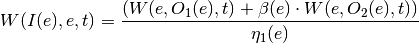
oemof.solph.linear_mixed_integer_constraints.add_variable_linear_eta_relation(model, block)[source]¶

Adds constraint for input-output relation for all units with variable efficiency grouped in block.objs.

The mathematical formulation for the constraint is as follows:

$W(I(e),e ,t) = Y(e,t) \cdot c_1 + c_2 \cdot W(e, O_1(e), t), \qquad \forall e, \forall t$

With $e \in E$ and $E$ beeing the set of unique ids for all entities grouped inside the attribute block.objs.

$O_1(e)$ beeing the set of all first outputs of entitiy (component) $e$ .

$I(e)$ beeing the set of all inputs of entitiy (component) $e$ .

Parameters:	model (OptimizationModel() instance) – An object to be solved containing all Variables, Constraints, Data. block (SimpleBlock()) –

oemof.solph.linear_mixed_integer_constraints.set_bounds(model, block, side='output')[source]¶

Set upper and lower bounds via constraints.

The bounds are set with constraints using the binary status variable of the components. The mathematical formulation is as follows:

If side is output:

$W(e, O_1(e), t) \leq out_{max}(e) \cdot Y(e, t), \qquad \forall e, \forall t$

$W(e, O_1(e), t) \geq out_{min}(e) \cdot Y(e, t), \qquad \forall e, \forall t$

If side is input:

$W(I(e), e, t) \leq in_{max}(e) \cdot Y(e, t), \qquad \forall e, \forall t$

$W(I(e), e, t) \geq in_{min}(e) \cdot Y(e, t), \qquad \forall e, \forall t$

With $e \in E$ and $E$ beeing the set of unique ids for all entities grouped inside the attribute block.objs.

$O_1(e)$ beeing the set of all first outputs of entitiy (component) $e$ .

$I(e)$ beeing the set of all inputs of entitiy (component) $e$ .

Parameters:	model (OptimizationModel() instance) – An object to be solved containing all Variables, Constraints, Data. Bounds are altered at model attributes (variables) of model block (SimpleBlock()) – side (string) – string to select on which side the bounds should be set (ìnput, output)

oemof.solph.objective_expressions module¶

The module contains different objective expression terms.

@author: Simon Hilpert (simon.hilpert@fh-flensburg.de)

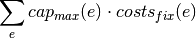
oemof.solph.objective_expressions.add_capex(model, block, ref='output')[source]¶

Add capital expenditure to linear objective.

If reference is output (e.g. powerplants):

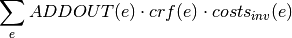
$\sum_e ADDOUT(e) \cdot crf(e) \cdot costs_{inv}(e)$

If reference is capacity (e.g. storages):

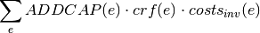
$\sum_e ADDCAP(e) \cdot crf(e) \cdot costs_{inv}(e)$

With $e \in E$ and $E$ beeing the set of unique ids for all entities grouped inside the attribute block.objs.

Parameters:	model (OptimizationModel() instance) – block (SimpleBlock()) – ref (string) – string to check if capex is referred to capacity (storage) or output (e.g. powerplant) Returns – --------- – Expression –

oemof.solph.objective_expressions.add_curtailment_costs(model, block=None)[source]¶

Cost term for dispatchable sources in linear objective.

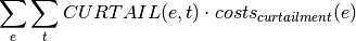
$\sum_e \sum_ t CURTAIL(e,t) \cdot costs_{curtailment}(e)$

With $e \in E$ and $E$ beeing the set of unique ids for all entities grouped inside the attribute block.objs.

Parameters:	model (OptimizationModel() instance) – block (SimpleBlock()) – Returns – --------- – Expression –

oemof.solph.objective_expressions.add_excess_slack_costs(model, block=None)[source]¶

Artificial cost term for excess slack variables.

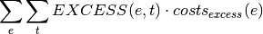
$\sum_e \sum_t EXCESS(e,t) \cdot costs_{excess}(e)$

With $e \in E$ and $E$ beeing the set of unique ids for all entities grouped inside the attribute block.objs.

Parameters:	model (OptimizationModel() instance) – block (SimpleBlock()) – Returns – --------- – Expression –

oemof.solph.objective_expressions.add_input_costs(model, block)[source]¶

Adds costs for usage of input (fuel, elec, etc. ) if not included in opex

$\sum_e \sum_t W(I(e), e, t) \cdot costs_{inflow}(e)$

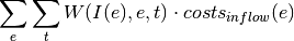
With $e \in E$ and $E$ beeing the set of unique ids for all entities grouped inside the attribute block.objs.

$I(e)$ beeing the set of all inputs of entitiy (component) $e$ .

Parameters:	model (OptimizationModel() instance) – An object to be solved containing all Variables, Constraints, Data. block (SimpleBlock()) – Returns – --------- – Expression –

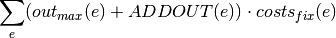
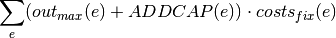
oemof.solph.objective_expressions.add_opex_fix(model, block, ref=None)[source]¶

Fixed operation expenditure term for linear objective function.

If reference is output (e.g. powerplants):

$\sum_e out_{max}(e) \cdot costs_{fix}(e)$

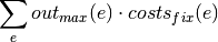
If reference is capacity (e.g. storages):

$\sum_e cap_{max}(e) \cdot costs_{fix}(e)$

If investment:

$\sum_e (out_{max}(e) + ADDOUT(e)) \cdot costs_{fix}(e)$

$\sum_e (out_{max}(e) + ADDCAP(e)) \cdot costs_{fix}(e)$

With $e \in E$ and $E$ beeing the set of unique ids for all entities grouped inside the attribute block.objs.

Parameters:	model (OptimizationModel() instance) – block (SimpleBlock()) – ref (string) – string to check if capex is referred to capacity (storage) or output (e.g. powerplant) Returns – --------- – Expression –

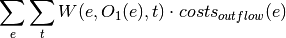
oemof.solph.objective_expressions.add_opex_var(model, block, ref='output')[source]¶

Variable operation expenditure term for linear objective function.

If reference of opex is output:

$\sum_e \sum_t W(e,O_1(e),t) \cdot costs_{outflow}(e)$

If reference of opex is input:

$\sum_e \sum_t W(I(e),e,t) \cdot costs_{inflow}(e)$

With $e \in E$ and $E$ beeing the set of unique ids for all entities grouped inside the attribute block.objs.

$O_1(e)$ beeing the set of all first outputs of entitiy (component) $e$ .

$I(e)$ beeing the set of all inputs of entitiy (component) $e$ .

Parameters:	model (OptimizationModel() instance) – An object to be solved containing all Variables, Constraints, Data. block (SimpleBlock()) – ref (string) – Reference side on which opex are based on (e.g. powerplant MWhth -> input or MWhel -> output) Returns – --------- – Expression –

oemof.solph.objective_expressions.add_ramping_costs(model, block, grad_direc='positive')[source]¶

Add gradient costs for components to linear objective expression.

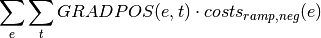
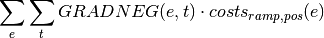
$\sum_e \sum_t GRADPOS(e,t) \cdot costs_{ramp,neg}(e)$

$\sum_e \sum_t GRADNEG(e,t) \cdot costs_{ramp,pos}(e)$

With $e \in E$ and $E$ beeing the set of unique ids for all entities grouped inside the attribute block.objs.

Parameters:	model (OptimizationModel() instance) – block (SimpleBlock()) – grad_direc (string) – direction of gradient for which the costs are added to the objective expression Returns – --------- – Expression –

oemof.solph.objective_expressions.add_revenues(model, block, ref='output')[source]¶

Revenue term for linear objective function.

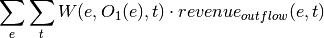
$\sum_e \sum_t W(e,O_1(e),t) \cdot revenue_{outflow}(e,t)$

With $e \in E$ and $E$ beeing the set of unique ids for all entities grouped inside the attribute block.objs.

$O_1(e)$ beeing the set of all first outputs of entitiy (component) $e$ .

Parameters:	model (OptimizationModel() instance) – block (SimpleBlock()) – Returns – --------- – Expression –

oemof.solph.objective_expressions.add_shortage_slack_costs(model, block=None)[source]¶

Artificial cost term for shortage slack variables.

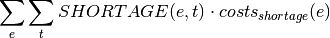
$\sum_e \sum_t SHORTAGE(e,t) \cdot costs_{shortage}(e)$

With $e \in E$ and $E$ beeing the set of unique ids for all entities grouped inside the attribute block.objs.

Parameters:	model (OptimizationModel() instance) – block (SimpleBlock()) – Returns – --------- – Expression –

oemof.solph.objective_expressions.add_shutdown_costs(model, block)[source]¶

Adds shutdown costs for components to objective expression

$\sum_{e} \sum_t Z_{stop}(e,t) \cdot costs_{stop}(e)$

Parameters:	model (OptimizationModel() instance) – block (SimpleBlock()) – Returns – --------- – Expression –

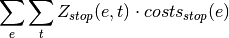
oemof.solph.objective_expressions.add_startup_costs(model, block)[source]¶

Adds startup costs for components to objective expression

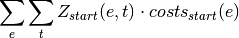
$\sum_{e} \sum_{t} Z_{start}(e,t) \cdot costs_{start}(e)$

With $e \in E$ and $E$ beeing the set of unique ids for all entities grouped inside the attribute block.objs.

Parameters:	model (OptimizationModel() instance) – block (SimpleBlock()) – Returns – --------- – Expression –

oemof.solph.optimization_model module¶

@contact Simon Hilpert (simon.hilpert@fh-flensburg.de)

class oemof.solph.optimization_model.OptimizationModel(energysystem)[source]¶

Bases: pyomo.core.base.PyomoModel.ConcreteModel

Create Pyomo model of the energy system.

Parameters:	entities (list with all entity objects) – timesteps (list with all timesteps as integer values) – options (nested dictionary with options to set.) –

default_assembler(block)[source]¶

Method for setting optimization model objects for blocks

Parameters:	self (OptimizationModel() instance) – block (SimpleBlock()) –

edges(components)[source]¶

Method that creates a list with all edges for the objects in components.

Parameters:	self – components (list of component objects) –
Returns:	edges
Return type:	list with tupels that represent the edges

objective_assembler(objective_options)[source]¶: calls functions to add predefined objective functions

results()[source]¶

Returns a nested dictionary of the results of this optimization model.

The dictionary is keyed by the Entities of the optimization model, that is om.results()[s][t] holds the time series representing values attached to the edge (i.e. the flow) from s to t, where s and t are instances of Entity.

Time series belonging only to one object, like e.g. shadow prices of commodities on a certain Bus, dispatch values of a DispatchSource or storage values of a Storage are treated as belonging to an edge looping from the object to itself. This means they can be accessed via om.results()[object][object].

Note that the optimization model has to be solved prior to invoking this method.

solve(solver='glpk', solver_io='lp', debug=False, duals=False, **kwargs)[source]¶

Method that takes care of the communication with the solver to solve the optimization model

Parameters:	self (pyomo.ConcreteModel) – str (solver_io) – str – or interface) 'lp','nl','python' ((file) – *kwargs (other arguments for the pyomo.opt.SolverFactory.solve()) – method* –
Returns:	self
Return type:	solved pyomo.ConcreteModel() instance

oemof.solph.optimization_model.assembler(e, om, block)[source]¶

Assemblers are the functions adding constraints to an optimization: model for a set of objects.

This is the most general form of assembler function, called only if no other, more specific assemblers have been found. Since we don’t know what to do in this case, we can only throw a TypeError.

Parameters:	entity (An object. Only used to figure out which assembler function to call) – by dispatching on its type. Not used otherwise. It’s a good idea to set this to None if the function is called directly via `assembler.registry`. om (The optimization model. Should be an instance of) – `pyomo.ConcreteModel`. block (A pyomo block.) –
Returns:	om – bus balances.
Return type:	The optimization model passed in as an argument, with additional

oemof.solph.predefined_objectives module¶

This module contains predefined objectives that can be used to model energy systems.

@author: Simon Hilpert (simon.hilpert@fh-flensburg.de)

oemof.solph.predefined_objectives.minimize_cost(self, cost_objects=None, revenue_objects=None)[source]¶

Builds objective function that minimises the total costs.

Costs included are:: opex_var, opex_fix, curtailment_costs (dispatch sources), annualised capex (investment components)

Parameters:	self (pyomo model instance) – cost_blocks (array like) – list containing classes of objects that are included in cost terms of objective function revenue_blocks (array like) – list containing classes of objects that are included in revenue terms of objective function

oemof.solph.variables module¶

Module contains variable definitions and constraint to bound variables (e.g. for investement).

@author: Simon Hilpert (simon.hilpert@fh-flensburg.de)

oemof.solph.variables.add_binary(model, block, relaxed=False)[source]¶

Creates all status variables (binary) for block.objs

Status variable indicates if a unit is turned on or off. E.g. if a transformer is switched on/off -> y=1/0

Parameters:	model (pyomo.ConcreteModel()) – A pyomo-object to be solved containing all Variables, Constraints, Data Variables are added as attributes to the model objs (array_like (list)) – all components for which the status variable is created relaxed (boolean) – If True “binary” variables will be created as continuous variables with bounds of 0 and 1.

oemof.solph.variables.add_continuous(model, edges)[source]¶

Adds all variables corresponding to the edges of the bi-partite graph for all timesteps.

The function uses the pyomo class Var() to create the optimization variables. As index-sets the provided edges of the graph (in general all edges) and the defined timesteps are used. If an invest model is used an additional optimization variable indexed by the edges is created to handle “flexible” upper bounds of the edge variable by using an additional constraint. The following variables are created: Variables for all the edges, variables for the state of charge of storages. (If specific components such as disptach sources and storages exist.)

Parameters:

model (OptimizationModel() instance) – A object to be solved containing all Variables, Constraints, Data Variables are added as attributes to the model
edges (array_like (list)) – edges will be a list containing tuples representing the directed edges of the graph by using unique ids of components and buses. e.g. [(‘coal’, ‘pp_coal’), (‘pp_coal’, ‘b_el’),...]

Returns:

The variables are added as a attribute to the optimization model object
model.

oemof.solph.variables.set_bounds(model, block, side='output')[source]¶

Sets bounds for variables that represent the weight of the edges of the graph if investment models are calculated.

For investment models upper and lower bounds will be modeled via additional constraints. The mathematical description for the constraint is as follows:

If side is output

$W(e, O_1(e)), t) \leq out_{max}(e, t), \qquad \forall e, \forall t$

With investment:

$W(e, O_1(e), t) \leq out_{max}(e, t) + ADDCAP(e,O_1[e]), \qquad \forall e, \forall t$

If side is input:

$W(I(e), e, t) \leq in_{max}(e, t), \qquad \forall e, \forall t$

With $e \in E$ and $E$ beeing the set of unique ids for all entities grouped inside the attribute block.objs.

$O_1(e)$ beeing the set of all first outputs of entitiy (component) $e$ .

$I(e)$ beeing the set of all inputs of entitiy (component) $e$ .

Parameters:	model (OptimizationModel() instance) – An object to be solved containing all Variables, Constraints, Data Constraints are added as attributes to the model block (SimpleBlock()) – side (string) – Side of component for which the bounds are set (‘input’ or ‘output’)

oemof.solph.variables.set_fixed_sink_value(model, block)[source]¶

Setting a value und fixes the variable of input.

The mathematical formulation is as follows:

$W(I(e), e,t) = val(e,t), \qquad \forall e, \forall t$

With $e \in E$ and $E$ beeing the set of unique ids for all entities grouped inside the attribute block.objs.

$I(e)$ beeing the set of all inputs of entitiy (component) $e$ .

Parameters:	model (OptimizationModel() instance) – An object to be solved containing all Variables, Constraints, Data Attributes are altered of the model block (SimpeBlock()) –

oemof.solph.variables.set_outages(model, block, outagetype='period', side='output')[source]¶

Fixes component input/output to zeros for modeling outages.

Parameters:

model (OptimizationModel() instance) – An object to be solved containing all Variables, Constraints, Data.
block (SimpeBlock()) –
outagetype (string) – Type to model outages of component if outages is scalar. ‘period’ yield one timeblock where component is off, while ‘random_days’ will sample random days over the timehorizon where component is off
side (string) – Side of component to fix to zero: ‘output’, ‘input’.

oemof.solph.variables.set_storage_cap_bounds(model, block)[source]¶

Alters/sets upper and lower bounds for variables that represent the absolut state of charge e.g. filling level of a storage component.

For investment models upper and lower bounds will be modeled via additional constraints. The mathematical description for the constraint is as follows:

$cap_{min}(e) \leq CAP(e, t) \leq cap_{max}(e), \qquad \forall e, \forall t$

If investment:

$CAP(e, t) \leq cap_{max}(e) + ADDCAP(e), \qquad \forall e, \forall t$

With $e \in E$ and $E$ beeing the set of unique ids for all entities grouped inside the attribute block.objs.

Parameters:	model (OptimizationModel() instance) – An object to be solved containing all Variables, Constraints, Data Bounds are altered at model attributes (variables) of model block (SimpleBlock()) –

Module contents¶

The solph-package contains funtionalities for creating and solving an optimizaton problem. The problem is created from oemof base classes. Solph depend on pyomo.