numkit.fitting — Fitting data
The module contains functions to do least square fits of functions of one variable f(x) to data points (x,y).
Example
For example, to fit a un-normalized Gaussian with FitGauss to
data distributed with mean 5.0 and standard deviation 3.0:
from numkit.fitting import FitGauss
import numpy, numpy.random

# generate suitably noisy data
mu, sigma = 5.0, 3.0
Y,edges = numpy.histogram(sigma*numpy.random.randn(10000), bins=100, density=True)
X = 0.5*(edges[1:]+edges[:-1]) + mu

g = FitGauss(X, Y)

print(g.parameters)
# [ 4.98084541  3.00044102  1.00069061]
print(numpy.array([mu, sigma, 1]) - g.parameters)
# [ 0.01915459 -0.00044102 -0.00069061]

import matplotlib.pyplot as plt
plt.plot(X, Y, 'ko', label="data")
plt.plot(X, g.fit(X), 'r-', label="fit")
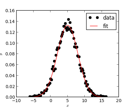
A Gaussian (red) was fit to the data points (black circles) with
the numkit.fitting.FitGauss class.
If the initial parameters for the least square optimization do not lead to a solution then one can provide customized starting values in the parameters keyword argument:
g = FitGauss(X, Y, parameters=[10, 1, 1])
The parameters have different meaning for the different fit functions; the documentation for each function shows them in the context of the fit function.
Creating new fit functions
New fit function classes can be derived from FitFunc. The
documentation and the methods FitFunc.f_factory() and
FitFunc.initial_values() must be overriden. For example, the
class FitGauss is implemented as
class FitGauss(FitFunc):
    '''y = f(x) = p[2] * 1/sqrt(2*pi*p[1]**2) * exp(-(x-p[0])**2/(2*p[1]**2))'''
    def f_factory(self):
        def fitfunc(p,x):
            return p[2] * 1.0/(p[1]*numpy.sqrt(2*numpy.pi)) * numpy.exp(-(x-p[0])**2/(2*p[1]**2))
        return fitfunc
    def initial_values(self):
        return [0.0,1.0,0.0]
The function to be fitted is defined in fitfunc(). The
parameters are accessed as p[0], p[1], ... For each parameter,
a suitable initial value must be provided.
Functions and classes
-
numkit.fitting.Pearson_r(x, y)¶ Pearson’s r (correlation coefficient).
Pearson(x,y) –> correlation coefficientx and y are arrays of same length.
- Historical note – Naive implementation of Pearson’s r ::
- Ex = scipy.stats.mean(x) Ey = scipy.stats.mean(y) covxy = numpy.sum((x-Ex)*(y-Ey)) r = covxy/math.sqrt(numpy.sum((x-Ex)**2)*numpy.sum((y-Ey)**2))
-
numkit.fitting.linfit(x, y, dy=None)¶ Fit a straight line y = a + bx to the data in x and y.
Errors on y should be provided in dy in order to assess the goodness of the fit and derive errors on the parameters.
linfit(x,y[,dy]) –> result_dictFit y = a + bx to the data in x and y by analytically minimizing chi^2. dy holds the standard deviations of the individual y_i. If dy is not given, they are assumed to be constant (note that in this case Q is set to 1 and it is meaningless and chi2 is normalised to unit standard deviation on all points!).
Returns the parameters a and b, their uncertainties sigma_a and sigma_b, and their correlation coefficient r_ab; it also returns the chi-squared statistic and the goodness-of-fit probability Q (that the fit would have chi^2 this large or larger; Q < 10^-2 indicates that the model is bad — Q is the probability that a value of chi-square as _poor_ as the calculated statistic chi2 should occur by chance.)
Returns: result_dict with components
- intercept, sigma_intercept
a +/- sigma_a
- slope, sigma_slope
b +/- sigma_b
- parameter_correlation
correlation coefficient r_ab between a and b
- chi_square
chi^2 test statistic
- Q_fit
goodness-of-fit probability
Based on ‘Numerical Recipes in C’, Ch 15.2.
-
class
numkit.fitting.FitFunc(x, y, parameters=None)¶ Fit a function f to data (x,y) using the method of least squares.
The function is fitted when the object is created, using
scipy.optimize.leastsq(). One must derive from the base classFitFuncand override theFitFunc.f_factory()(including the definition of an appropriate localfitfunc()function) andFitFunc.initial_values()appropriately. See the examples for a linear fitFitLin, a 1-parameter exponential fitFitExp, or a 3-parameter double exponential fitFitExp2.- The object provides two attributes
FitFunc.parameters- list of parameters of the fit
FitFunc.message- message from
scipy.optimize.leastsq()
After a successful fit, the fitted function can be applied to any data (a 1D-numpy array) with
FitFunc.fit().-
f_factory()¶ Stub for fit function factory, which returns the fit function. Override for derived classes.
-
fit(x)¶ Applies the fit to all x values
-
initial_values()¶ List of initital guesses for all parameters p[]
-
class
numkit.fitting.FitLin(x, y, parameters=None)¶ y = f(x) = p[0]*x + p[1]
-
class
numkit.fitting.FitExp(x, y, parameters=None)¶ y = f(x) = exp(-p[0]*x)
-
class
numkit.fitting.FitExp2(x, y, parameters=None)¶ y = f(x) = p[0]*exp(-p[1]*x) + (1-p[0])*exp(-p[2]*x)
-
class
numkit.fitting.FitGauss(x, y, parameters=None)¶ y = f(x) = p[2] * 1/sqrt(2*pi*p[1]**2) * exp(-(x-p[0])**2/(2*p[1]**2))
Fits an un-normalized gaussian (height scaled with parameter p[2]).
- p[0] == mean $mu$
- p[1] == standard deviation $sigma$
- p[2] == scale $a$