Using Epigrass

To simulate an epidemic process in Epigrass, the user needs to have in hand at least three files: Two files containing the site and edge data and a third file which is a script that defines what it is to be done. Here we go through each one of them in detail. The last part of this chapter is a step-by step guide the Graphical User Interface (GUI).

Data

Site data file

See below an example of the content of a site file for a network of 10 cities. Each line corresponds to a site (except the first line which is the title). For each site, it is declared, in this order: its spatial location in the form of a pair of coordinates ([X,Y]); a site $name$ to be used in the output; the site’s population; the site geocode (an arbitrary unique number which is used internally by Epigrass).

X	Y	City	Pop	Geocode
1	4	“N1”	1000000	1
2	4	“N2”	100000	2
3	4	“N3”	1000	3
4	4	“N4”	1000	4
5	4	“N5”	1000	5
1	3	“N6”	100000	6
2	3	“N7”	1000	7
3	3	“N8”	100000	8
4	3	“N9”	100000	9
5	3	“N10”	1000	10
1	2	“N11”	1000	11

In this example, the first site is located at [X,Y]=[1,4], it is named N1, its population is 1000000 and its geocode is 1. This is minimum configuration of a site data file and it must contains this information in exactly this order.

In some situations, the user may want to add other attributes to the sites (different transmission parameters, or vaccine coverage or initial conditions for simulations). This information is provided by adding new columns to the minimum file. For example, if one wishes to add information on the vaccine coverage in cities N1 to N10 ($vac$) as well as information about average temperature (which hypothetically affects the transmission of the disease), the file becomes:

X	Y	City	Pop	Geocode	Vac	Temp
1	4	“N1”	1000000	1	0.9	32
2	4	“N2”	100000	2	0.88	29
3	4	“N3”	1000	3	0.7	25
4	4	“N4”	1000	4	0.2	34
5	4	“N5”	1000	5	0	26
1	3	“N6”	100000	6	0	27
2	3	“N7”	1000	7	0	31
3	3	“N8”	100000	8	0	30
4	3	“N9”	100000	9	0	24
5	3	“N10”	1000	10	0	31

During the simulation, each site object receives these informations and store them in appropriate variables that can be used later during model specification. Population is stored in the variable N; while the extra columns (those beyond the geocode) are stored in a tuple named {values. For example, for the city N1, we have N = 1000000 and values=[0.9,32]. During model specification, we may use N to indicate the population size and/or we can use values[0] to indicate the level of vaccination of that city and values[1] to indicate the temperature.

It is up to the user, to know what means the elements of the tuple values. Note that the first element of the tuple has index 0,the second one has index 1 and so on.

When using real data, one may wish to use actual geocodes and coordinates. For example, for a network of Brazilian cities, one may build the following file:

latitude	longitude	local	pop	geocode
-16:19:41	-48:57:10	ANAPOLIS	280164	520110805
-10:54:32	-37:04:03	ARACAJU	461534	280030805
-21:12:27	-50:26:24	ARACATUBA	164449	350280405
-18:38:44	-48:11:36	ARAGUARI	92748	310350405
-21:13:17	-43:46:12	BARBACENA	103669	310560805
-22:32:53	-44:10:30	BARRA_MANSA	165134	330040705
-20:33:11	-48:34:11	BARRETOS	98860	350550005
-26:54:55	-49:04:15	BLUMENAU	241943	420240405
-22:57:09	-46:32:30	B.PAULISTA	111091	350760505

In this file, the coordinates are the actual geographical latitude and longitude coordinates. This information is important when using Epigrass with a map in shapefile format. The geocode is also the official geocode of these localities (the same one used in the shapefile). Despite the cumbersome size of the number, it may be worth using it because demographic official databases are often linked by this number.

Edge data file

The edge data file contains all the direct links between sites. Each line in the file (except for the first, which is the header) corresponds to an edge. For each edge (or link) one must specify (in this order): the names of the sites connected by that edge; the number of individuals traveling from source to destination; the number of individuals travelling from destination to source per time step; the distance or length of the edge. At last, the file must contain, in the fifth and sixth columns, the geocodes of the source and destination sites*. This is very important as the graph is built internally connecting sites through edges and this is done based on geocode info.

Warning

It is required that the order of columns is kept the same.

See below the list of the 8 edges connecting the sites N1 to N10. Let’s look the first one, as an example. It links N1 to N2. Through this link passes 11 individuals backwards and forwards per time step (a day, for example). This edge has length 1 (remember that N1 is at [X,Y]=[1,1] and N2 is at [X,Y]=[1,2], so the distance between them is 1). The last two columns show the geocode of N1 (geocode 1) and the geocode of N2 (geocode 2).

Source	Dest	flowSD	flowDS	Distance	geoSource	geoDest
N1	N2	11	11	1	1	2
N2	N4	0.02	0.02	1	3	4
N3	N8	1.01	1.01	1	3	8
N4	N9	1.01	1.01	1	4	9
N5	N10	0.02	0.02	1	5	10
N6	N5	1.01	1.01	1	7	8
N7	N10	1.01	1.01	1	7	8
N9	N10	1.01	1.01	1	9	10

Note that it doesn’t matter which site is considered a Source and which one is considered a Destination. I.e., if there is a link between A and B, one may either named A as source and B as destination, or the other way around.

If the edge represents a road or a river, one may use the actual metric distance as length. If the edge links arbitrary localities, one may opt to use euclidean distance, calculated from the x and y coordinates (using Pythagoras theorem).

Specifying a model: the script

Once the user has specified the two data files, the next step is to define the model to be executed. This is done in the .epg script file. The .epg script is a text file and can be edited with any editor (not word processor). This script must be prepared with care.

The best way to write down your own .epg is to edit an already existing .epg file. So, open Epigrass, choose an .epg file and click on the Edit button. Your favorite editor will open and you can start editing. Don’t forget to save it as a new file in your working directory. Of course, there is an infinite number of possibilities regarding the elaboration of the script. It all depends on the goals of the user.

Note

Another way to edit an .epg file is to open it whith the graphical editor provided with Epigrass. Just type epgeditor yourmodel.epg.

For the beginner, we suggest him/her to take a look at the .epg files in the demo directory. They are all commented and may help the user in getting used with Epigrass language and capabilities.

Some hints to be successful when editing your .epg:

• All comments in the script are preceded by the symbol #. These comments may be edited by the user as he/she wishes and new lines may be added at will. Don’t forget, however, to place the symbol # in every line corresponding to a comment.
• The script is divided into a few parts. These parts have capital letter titles within brackets. Don’t touch them!
• Don’t remove any line that is not a comment. See below how to appropriately edit these command lines.

Let’s take a look now at each part of a script (this is the script .epg demo file):

Warning

All variables defined in a .epg are case-insensitive. Consider this fact when naming your model’s variables.

Part 1: THE WORLD

The first section of the script is titled: THE WORLD. An example of its content is shown:

shapefile = ['riozonas_LatLong.shp','nome_zonas','zona_trafe']
edges = edges.csv
sites = sites.csv
encoding =

where,

shapefile

Is a list with 3 elements: the first is the path, relative to the working directory, of the shapefile file; the second is the variable, in the shapefile, which contains the names of the localities (polygons of the map); the third and last is the variable, in the shapefile, which contains the geocode of the localities. If you don’t have a map for you simulation, leave the list empty: location = [] ).

edges

This is the name of the .CSV (comma-separated-values) file containing the list of edges and their attributes.

sites

This is the name of the .CSV file containing the list of sites and their attributes.

encoding

This is the encoding used in your sites and edges files. This is very important when you use location names which include non-ascii characters. The default encoding is latin-1. If you use any other encoding, please specify it here. Example: utf-8.

Note

All paths in the .epg file are relative to the working directory.

Part 2: EPIDEMIOLOGICAL MODEL

This is the main part of the script. It defines the epidemiological model to be run. The script reads:

modtype = SIR

Here, the type of epidemiological model is defined, in this case is a deterministic SIR model. Epigrass has some built-in models:

Name	Determ.	Stochastic
Susceptible-Infected-Recovered	SIR	SIR_s
Susceptible-Exposed-Infected-Recovered	SEIR	SEIR_s
Susceptible-Infected-Susceptible	SIS	SIS_s
Susceptible-Exposed-Infected-Susceptible	SEIS	SEIS_s
SIR with fraction with full immunity	SIpRpS	SIpRpS_s
SEIR with fraction with full immunity	SEIpRpS	SEIpRpS_s
SIR with partial immunity for all	SIpR	SIpR_s
SEIR with partial immunity for all	SEIpR	SEIpR_s
SIR with immunity wane	SIRS	SIRS_s

A description of these models can be found in the chapter Epidemiological modeling. The stochastic models use Poisson distribution as default for the number of new cases (L(t+1)). Besides these, the user may define his/her own model and access by the protect word Custom.

Part 3: MODEL PARAMETERS

The epidemic model is defined by variables and parameter which require initialization:

#==============================================================#
    #  They can be specified as constants or as functions of global or
    #  site-specific variables. Site-specific variables are provided
    #  in the sites .csv file. In this file, all columns after the 4th
    #  are collected into a values tuple, which can be referenced here
    #  as values[0], values[1], values[2], etc.
    #   Examples:
    #   beta = 0.001
    #   beta=values[0] #assigns the first element of values to beta
    #   beta=0.001*values[1]
    #   beta=0.001*N  # N is a global name for total site population
    # Currently, Epigrass requires that parameters beta, alpha, e, r, delta, B, w, p
    # be present in the .epg even if they will not be used. Do not erase these lines.
    # Just disregard them if they are not useful to you.

beta = 0.4   #transmission coefficient (contact rate * transmissibility)
alpha = 1  # clumping parameter
e = 1   # inverse of incubation period
r = 0.1   # inverse of infectious period
delta = 1  # probability of acquiring full immunity [0,1]
B = 0           # Birth rate
w = 0           # probability of immunity waning [0,1]
p = 0           #

These are the model parameters. Not all parameters are necessary for all models. For example, e is only required for SEIR-like models. Don’t remove the line, however because that will cause an error. We recommend that, if the parameter is not necessary, just add a comment after it as a reminder that it is not being used by the model.

In some cases, one may wish to assign site-specific parameters. For example, transmission rate may be different between localities that are very distant and are exposed to different climate. In this case site specific variables can be added as new columns to the site file. All columns after the geocode are packed into a tuple named values and can be referenced in the order they appear. I.e., the first element of the tuple is values[0], the second element is values[1], the third element is values[2] and so on.

Part 4: INITIAL CONDITIONS

In this part of the script, the initial conditions are defined. Here, the number of individuals in each epidemiological state, at the start of the simulation, is specified. It reads:

#==============================================================#
# Here, the number of individuals in each epidemiological
# state (SEI) is specified. They can be specified in absolute
# or relative numbers.
# N is the population size of each site.
# The rule defined here will be applied equally to all sites.
# For site-specific definitions, use EVENTS (below)
# Examples:
#   S,E,I = 0.8*N, 10, 0.5*N
#   S,E,I = 0.5*N, 0.01*N, 0.05*N
#   S,E,I = N-1, 1, 0
S = N
E = 0
I = 0

Here, N is the total population in a site (as in the datafile for sites). In this example, we set all localities to the same initial conditions (all individuals susceptible) and use an event (see below) to introduce an infectious individual in a locality. The number of recovered individuals is implicit, as R = N-(S+E+I)

Another possibility is to define initial conditions that are different for each site. For this, the data must be available as extra columns in the site data file and these columns are referenced to using the values tuple explained above.

Part 5: EPIDEMIC EVENTS

The next step is to define events that will occur during the simulation. These events may be epidemiological (arrival of an infected, for example) or a public health action (vaccination campaign, for example):

#=============================================================#
#   Specify isolated events.
#   Localities where the events are to take place should be Identified by the geocode, which
#  comes after population size on the sites data file.
#  All coverages must be a number between 0 and 1.
#  Seed : [('locality1's geocode',epid state, n),('locality2's geocode', epid state, n),...]
#  N infected cases will be added to locality at time 0.
#  Vaccinate: [('locality1's geocode', [t1,t2,...], [cov1,cov2,...]),('locality2's geocode', [t1,t2,...], [cov1,cov2,...])]
#  Quarantine: [(locality1's geocode,time,coverage), (locality2's geocode,time,coverage)]
#seed = [(4550601,'ip20',10)] #santo cristo  #
seed = [(4552110,'ip20',10)] #pechincha  #
#seed = []
Vaccinate = [] #
Quarantine = []

The events currently implemented are:

seed

One or more infected individual(s) are introduced into a site, at the beggining of the simulation. The notation for a single event is: Seed = [(‘locality1’s geocode’,epid state, n),(‘locality2’s geocode’, epid state, n),...]. For example, seed = [(2,’I’,10)] programs the arrival of 10 infected individuals at site geocode 2, at time 1.

Vaccinate

Implements a campaign that vaccinates a fraction of the population in a site, at a pre-defined time-step. For multiple events, the notation is: [(‘locality1’s geocode’, [t1,t2,...], [cov1,cov2,...]),(‘locality2’s geocode’, [t1,t2,...], [cov1,cov2,...])], where the first element of every triplet is the geocode of the city, the second element is a list of the time(s) when the campaign is carried on, and the third element is the coverage(s). For example, the event [(2,[10],[0.7])] means that city 2, at time 10, has 70% of its population vaccinated. Mathematically, it means (in the model), the removal of individuals from the susceptible to the recovered stage.

Quarantine

Prevents any individual from leaving a site, starting at t. Currently disabled.

Part 6: TRANSPORTATION MODEL

Here, there are two options regarding the movement of infected individuals from site to site (through the edges). If stochastic = 0, the process is simulated deterministically. The number of infected passengers commuting through an edge is a fraction p of the infected population that is traveling. p is calculated as total passengers/total population.

If stochastic = 1, the number of passengers is sampled from a Poisson distribution with parameter given by the expected number of travelling infectives (calculated as above):

#=========================================================#
# If doTransp = 1 the transportation dynamics will be
# included. Use 0 here only for debugging purposes.
doTransp = 1

# Mechanism can be stochatic (1) or deterministic(0).
stochastic = 1
#Average speed of transportation system in km per time step. Enter 0 for instantaneous travel.
#Distance unit must be the same specified in edges files
speed =0 #1440  km/day -- equivalent to 60 km/h

That ends the definition of the model.

Part 7: SIMULATION AND OUTPUT

Now it is time to define some final operational variables for the simulation:

#==============================================================#
# Number of steps
steps = 50

# Output dir. Must be a full path. If empty the output will be generated on the
# same path as the model script.
outdir =

# Output file
outfile = simul.dat

# Database Output
# MySQLout can be 0 (no database output) or 1
MySQLout = 1


# Report Generation
# The variable report can take the following values:
# 0 - No report is generated.
# 1 - A network analysis report is generated in PDF Format.
# 2 - An epidemiological report is generated in PDF Format.
# 3 - A full report is generated in PDF Format.
# siteRep is a list with site geocodes. For each site in this list, a detailed report is apended to the main report.
report = 0
siteRep = []

# Replicate runs
# If replicas is set to an integer(n) larger than zero, the model will be run
# n times and the results will be consolidated before storing.
# RandSeed = 1: the seed will be randomized on each replicate
# RandSeed = 2: seeds are taken sequentially from the site's file
# Note: Replicate mode automatically turn off report and batch options.
Replicas = 10
RandSeed = 2
#Batch Run
#  list other scripts to be run in after this one. don't forget the extension .epg
#  model scripts must be in the same directory as this file or provide full path.
#  Example: Batch = ['model2.epg','model3.epg','/home/jose/model4.epg']
Batch = []#['sarsDF.epg','sarsPA.epg','sarsRS.epg']

where,

step

Number of time steps for the simulation.

outdir

Directory for data output (currently not in use)

outfile

.csv filename that can be imported into R as a dataframe. This .csv file contains the simulated timeseries for all nodes.

MySQLout

Use MySQLout = 1 if simulated time series are to be stored in MySQL database. Time series of L, S, E, and I, from simulations, are stored in a MySQL database named epigrass. The results of each individual simulation is stored in a different table named after the model’s script name, the date and time the simulation has been run. For instance, suppose you run a simulation of a model stored in a file named script.epg, then at the end of the simulation, a new table in the epigrass database will be created with the following name: script_Wed_Jan_26_154411_2005. Thus, the results of multiple runs from the same model get stored independently.

Batch=[]

Script files included in this list are executed after the currently file is finished.

The Graphical User Interface(GUI)

Epigrass comes with a simple but effective GUI, that allows the user to control some aspects of the run-time behavior of the system. The Gui can be invoked by typing texttt{epigrass} in prompt of a console. We suggest the user to start Epigrass from the same directory where his/her model definition is located (.csv and .epg files).

All the information that is entered via the GUI gets stored in a hidden file called texttt{.epigrassrc} stored in the home folder of the user. Every time the GUI is invoked, the data stored in the texttt{.epigrassrc} file is used to fill the forms in the GUI. The gui is designed as a tabbed notebook with four tabs (Run Options, Settings, Utilities, and Visualization).

At the bottom of the Gui there are three buttons Help, Start and Exit. Their functions will be explained below. Immediately above the Run and Exit buttons, there is a small numeric display that will display the simulation progress after it has been started.

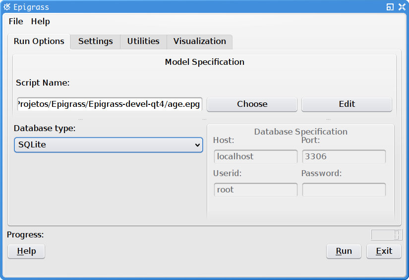
First tab of Epigrass GUI. This is where you setup your database output settings and the model to be run.

Run Options

The first tab of the GUI, contains a number of variables that, with the exception of the model script filename, should remain the same for most simulations you are going to run.

On the top of the first tab is a text box to enter the file name of the model script (something.epg). By clicking on the Choose button at the right of this box, you get a file selection dialog to select your script file. If you need you can click on the Edit button below to edit the script file with your favorite text editor.

Below, you can enter details about the MySQL database that will store the output of your simulations. Here you can enter the server IP, port, user and password. On the first time you run the GUI these input boxes will be filled with the default values for these variables (server on localhost, port 3306, user epigrass and password epigrass)

Settings

On the settings page, you can enter personal details such as user name (To be used in the simulation report), preferred text editor and preferred PDF reader. The preferred text editor will be used to open your script from the GUI, when you click on the edit button in the first tab. The PDF reader specified, will be used to open the report file, when requested (Utilities tab) and the user manual, when the user clicks on the help button on the bottom-left corner of the GUI.

On this tab, the language of the GUI can also be selected from a list of available translations. The effects of language changes will only take place when the next time the GUI is started.

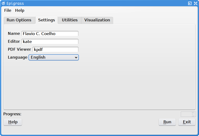
Settings tab of the Epigrass GUI. This is wher you configure the behavior os the GUI. Values set here will be remembered on future runs.

Utilities

In the Utilities tab, you can get feed back from the simulator. Especially during long simulation runs, it is good to know how it is progressing. During the simulation, text messages regarding the status of the simulation are written to the text box on the left.

On the right, there is a button for backing up the data base and another for opening the report generated by the last simulation. Since report PDFs ar stored in folder directly below the ones on which the simulation is started, older reports should still be accessible and can be opened directly by selecting the desired report using the operating system’s file manager.

Visualization

The fourth tab of the GUI is the visualization Tab. This tab was designed for playing animations of any simulation data that is stored in the database. Pressin the Scan DB button, causes the available tables in the epigrass database to be listed in the Simulations stored combo box. The user can then select one of these simulations to visualize. Once the simulation is selected the Variable to display combo-box will fill-up with the variables in the table devoted to the simulation. Select a variable.

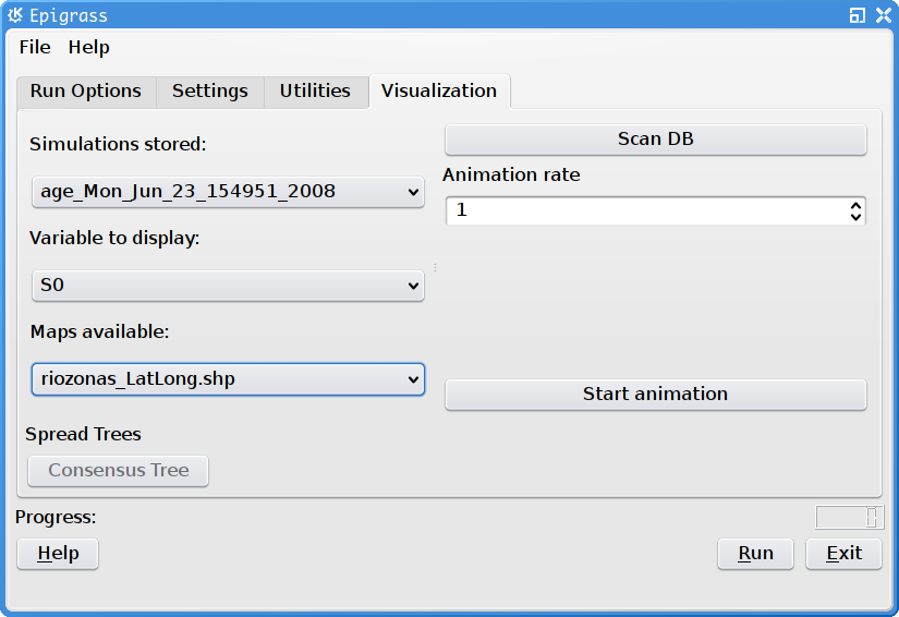
Visualization tab of the Epigrass GUI. The simulations and varibales to inspect are chosen here.

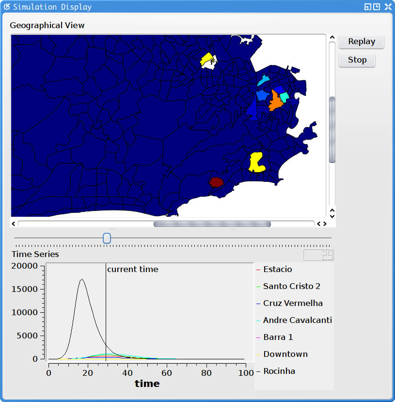
Once the Start animation button is pressed, a graphical display window pops up, and the simulation results will be displayed as a map or a graph (if no map was specified at the .epg). The animation can be replayed or moved to any timestep by dragging on the slider under the display widget. When the user moved the mouse over a polygon in the map(or node in the graph) its name and geocode appears as a tooltip. Polygons (nodes) can be selected with the mouse to display their full time series in the plot below the top display widget.

Operation

For running simulations, after all the information has been entered and checked on the first tab of the GUI, you can press the Run button to start the simulation or the :guilabel`Exit` button. When the Run button is pressed, the ~/.epigrassrc file is updated with all the information entered in the GUI. If the Exit button is pressed, all information entered since the last time the Run button was pressed is lost.

Epigrass also allows running simulation straight from the command line, with the epirunner executable. all you have to do is:

$ epirunner mymodel.epg

and the model will executed with the settings specified in the ~/.epigrassrc file. for help with epirunner, type:

$ epirunner -h
Usage: epirunner [options] your_model.epg

Options:
  --version             show program's version number and exit
  -h, --help            show this help message and exit
  -b <mysql|sqlite|csv>, --backend=<mysql|sqlite|csv>
                                                Define which datastorage backend to use
  -u DBUSER, --dbusername=DBUSER
                                                MySQL user name
  -p DBPASS, --password=DBPASS
                                                MySQL password for user
  -H DBHOST, --dbhost=DBHOST
                                                MySQL hostname or IP address