Differentiation of ODE Solvers

It is easy to use AD techniques to differentiate time integrations schemes, e.g. for Ordinary Differential Equations (ODEs) or Differential Algebraic Equations (DAEs). Here we illustrate the approach at ODE solvers. For simplicity we treat the explict Euler and the implicit Euler. These two schemes already already show many aspects that can also be found in more sophisticated solvers. For a details discussion see [Eberhard99] and dedicated software for semi-implicit DAEs SolvIND.

The goal is to compute derivatives of the form \(\frac{d x(t)}{d p}\), where \(x(t) \equiv x(t; x_0, p) \in \mathbb R^{N_x}\) is solution of the ordinary differential equation

\[\begin{split}\dot x(t) = f(t, x, p) \\ x(0) = x_0(p) \;,\end{split}\]

where the initial values \(x(0)\) is a function \(x_0(p)\) depending on some parameter \(p \in \mathbb R^{N_p}\).

Consider the following code that computes \(\frac{d x(t)}{d p}\) of the harmonic oscillator described by the ODE

\[\begin{split}\dot x(t) = \begin{pmatrix} x_2 \\ -p x_1 \end{pmatrix} \;.\end{split}\]

Explict Euler

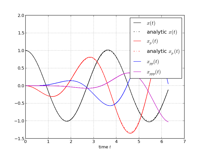
To illustrate the idea, we use the explict Euler integration scheme.

import numpy; from numpy import sin,cos; from algopy import UTPM, zeros
D,P = 4,1
x = UTPM(numpy.zeros((D,P,2)))
x.data[0,:,0] = 1
p = UTPM(numpy.zeros((D,P)))
p.data[0,:] = 3; p.data[1,:] = 1

def f(x):
    retval = x.zeros_like()
    retval[0] = x[1]
    retval[1] = -p* x[0]
    return retval

# compute AD solution
ts = numpy.linspace(0,2*numpy.pi,2000)
x_list = [x.data.copy() ]
for nts in range(ts.size-1):
    h = ts[nts+1] - ts[nts]
    x = x + h * f(x)
    x_list.append(x.data.copy())

# analytical solution
def x_analytical(t,p):
    return numpy.cos(numpy.sqrt(p)*t)
    
def x_p_analytical(t,p):
    return -0.5*numpy.sin(numpy.sqrt(p)*t)*p**(-0.5)*t

xs = numpy.array(x_list)
print(xs.shape)
import matplotlib.pyplot as pyplot; import os
pyplot.plot(ts, xs[:,0,0,0], ',k-', label = r'$x(t)$')
pyplot.plot(ts, x_analytical(ts,p.data[0,0]), 'k-.', label = r'analytic $x(t)$')
pyplot.plot(ts, xs[:,1,0,0], ',r-', label = r'$x_p(t)$')
pyplot.plot(ts, x_p_analytical(ts,p.data[0,0]), 'r-.', label = r'analytic $x_p(t)$')
pyplot.plot(ts, xs[:,2,0,0], ',b-', label = r'$x_{pp}(t)$')
pyplot.plot(ts, xs[:,3,0,0], ',m-', label = r'$x_{ppp}(t)$')



pyplot.xlabel('time $t$')
pyplot.legend(loc='best')
pyplot.grid()
pyplot.savefig(os.path.join(os.path.dirname(os.path.realpath(__file__)),'explicit_euler.png'))
# pyplot.show()
    

Implicit Euler

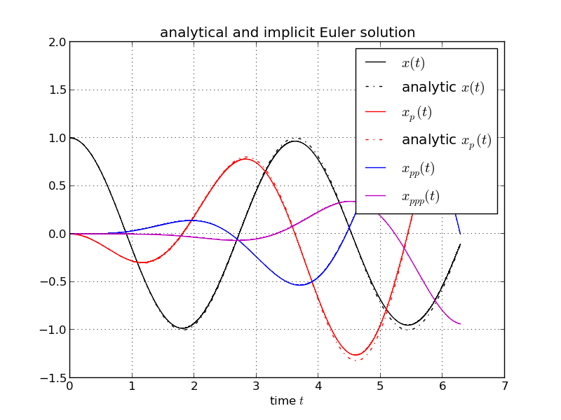
Since in practice often implicit integration schemes (stiff ODEs) are necessary, we illustrate the approach at the example of the implicit Euler integration scheme:

The ODE is discretized in time as

\[\begin{split}x_{k+1} - x_k = (t_{k+1} - t_k) f(t_{k+1}, x_{k+1}, p) \\ 0 = F(x_{k+1}, x_k, t_{k+1}, t_k, p) = (t_{k+1} - t_k) f(t_{k+1}, x_{k+1}, p) - x_{k+1} + x_k\end{split}\]

The task at hand is to solve this implicit function in UTP arithmetic, i.e. given \(0 = F(x,y)\), where \(x\) is input and \(y\) is output, solve

\[0 = F([x]_D, [y]_D) \mod T^D \;.\]

There are several possibilities to achieve this goal. For instance one can first solve the nominal problem \(0 = F(x,y)\) then successively compute the higher-order coefficients \(y_d, d=1,\dots,D-1\). To soution of the nominal problem can be done by applying Newton’s method, i.e. given an initial guess for \(y\) compute an update \(\delta y\), i.e. iterate

\[\begin{split}\delta y = - (F_x(x,y))^{-1} F(x,y) \\ y = y + \delta y\end{split}\]

Once \(y\) is known one can find the higher-order coefficients by using Newton-Hensel lifting

\[y_d T^d = -(F_x(x,y))^{-1} F([y]_{d}, [x]_{d+1}) \mod T^{d+1} \;.\]

The complete procedure is shown in the following code:

import numpy; from numpy import sin,cos; from algopy import UTPM, zeros
D,P = 4,1
x = UTPM(numpy.zeros((D,P,2)))
x.data[0,:,0] = 1
p = UTPM(numpy.zeros((D,P)))
p.data[0,:] = 3; p.data[1,:] = 1

def f(t, x, p):
    retval = x.copy()
    retval[0] = x[1]
    retval[1] = -p* x[0]
    return retval
    
def implicit_euler(f_fcn, x0, ts, p):
    """ implicit euler with fixed stepsizes, using Newton's method to solve
    the occuring implicit system of nonlinear equations
    """
    
    def F_fcn(x_new, x, t_new, t, p):
        """ implicit function to solve:  0 = F(x_new, x, t_new, t_old)"""
        return (t_new - t) * f_fcn(t_new, x_new, p) - x_new + x
        
    def J_fcn(x_new, x, t_new, t, p):
        """ computes the Jacobian of F_fcn
        all inputs are double arrays
        """
        y = UTPM(numpy.zeros((D,N,N)))
        y.data[0,:]   = x_new
        y.data[1,:,:] = numpy.eye(N)
        F = F_fcn(y, x, t_new, t, p)
        return F.data[1,:,:].T
        
        
    x = x0.copy()
    D,P,N = x.data.shape
    x_new = x.copy()

    x_list = [x.data.copy() ]
    for nts in range(ts.size-1):
        h = ts[nts+1] - ts[nts]
        x_new.data[0,...] = x.data[0,...]
        x_new.data[1:,...] = 0

        # compute the Jacobian at x
        J = J_fcn(x_new.data[0,0], x.data[0,0], ts[nts+1], ts[nts], p.data[0,0])

        # d=0: apply Newton's method to solve 0 = F_fcn(x_new, x, t_new, t)
        step = numpy.inf
        while step > 10**-10:
            delta_x = numpy.linalg.solve(J, F_fcn(x_new.data[0,0], x.data[0,0], ts[nts+1], ts[nts], p.data[0,0]))
            x_new.data[0,0] -= delta_x
            step = numpy.linalg.norm(delta_x)
        
        # d>0: compute higher order coefficients
        J = J_fcn(x_new.data[0,0], x.data[0,0], ts[nts+1], ts[nts], p.data[0,0])
        for d in range(1,D):
            F = F_fcn(x_new, x, ts[nts+1], ts[nts], p)
            x_new.data[d,0] = -numpy.linalg.solve(J, F.data[d,0])
        
        x.data[...] = x_new.data[...]
        x_list.append(x.data.copy())
        
    return numpy.array(x_list)
    

# compute AD solution
ts = numpy.linspace(0,2*numpy.pi,1000)
xs = implicit_euler(f, x, ts, p)

# print xs
# analytical solution
def x_analytical(t,p):
    return numpy.cos(numpy.sqrt(p)*t)
    
def x_p_analytical(t,p):
    return -0.5*numpy.sin(numpy.sqrt(p)*t)*p**(-0.5)*t

print(xs.shape)
import matplotlib.pyplot as pyplot; import os
pyplot.plot(ts, xs[:,0,0,0], ',k-', label = r'$x(t)$')
pyplot.plot(ts, x_analytical(ts,p.data[0,0]), 'k-.', label = r'analytic $x(t)$')
pyplot.plot(ts, xs[:,1,0,0], ',r-', label = r'$x_p(t)$')
pyplot.plot(ts, x_p_analytical(ts,p.data[0,0]), 'r-.', label = r'analytic $x_p(t)$')
pyplot.plot(ts, xs[:,2,0,0], ',b-', label = r'$x_{pp}(t)$')
pyplot.plot(ts, xs[:,3,0,0], ',m-', label = r'$x_{ppp}(t)$')

pyplot.title('analytical and implicit Euler solution')
pyplot.xlabel('time $t$')
pyplot.legend(loc='best')
pyplot.grid()
pyplot.savefig(os.path.join(os.path.dirname(os.path.realpath(__file__)),'implicit_euler.png'))
# pyplot.show()
     

The generated plot shows the numerically computed trajectory and the analytically derived solutions. One can see that the numerical trajectory of \(\frac{d x(t)}{d p}\) is close to the analytical solution. More elaborate ODE integrators would yield better results.

[Eberhard99]

Automatic Differentiation of Numerical Integration Algorithms, http://www.jstor.org/pss/2585052