Minimal Surface Problem

In this example it is shown how the gradient of the function

def O_tilde(u):
    """ this is the objective function"""
    M = numpy.shape(u)[0]
    h = 1./(M-1)
    return M**2*h**2 + numpy.sum(0.25*( (u[1:,1:] - u[0:-1,0:-1])**2 + (u[1:,0:-1] - u[0:-1, 1:])**2))

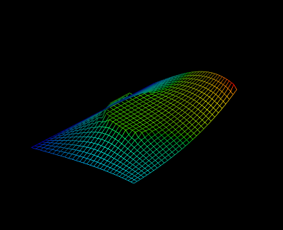
can be computed conveniently using ALGOPY. It is the objective function of a minimal surface problem. With boundary constraints and an additional constraint in the domain in form of a cylinder one obtains a plot like

At first the initial values are specified and the function evaluation is traced

# INITIAL VALUES
M = 30
h = 1./M
u = numpy.zeros((M,M),dtype=float)
u[0,:]=  [numpy.sin(numpy.pi*j*h/2.) for j in range(M)]
u[-1,:] = [ numpy.exp(numpy.pi/2) * numpy.sin(numpy.pi * j * h / 2.) for j in range(M)]
u[:,0]= 0
u[:,-1]= [ numpy.exp(i*h*numpy.pi/2.) for i in range(M)]

# trace the function evaluation and store it in cg
cg = algopy.CGraph()
Fu = algopy.Function(u)
Fy = O_tilde(Fu)
cg.trace_off()
cg.independentFunctionList = [Fu]
cg.dependentFunctionList = [Fy]

One can now compute the gradient of the objective function as follows

def dO_tilde(u):
    # use ALGOPY to compute the gradient
    g = cg.gradient([u])[0]

    # on the edge the analytical solution is fixed
    # so search direction must be zero on the boundary

    g[:,0]  = 0
    g[0,:]  = 0
    g[:,-1] = 0
    g[-1,:] = 0
    return g

The complete code is

import numpy
import algopy

def O_tilde(u):
    """ this is the objective function"""
    M = numpy.shape(u)[0]
    h = 1./(M-1)
    return M**2*h**2 + numpy.sum(0.25*( (u[1:,1:] - u[0:-1,0:-1])**2 + (u[1:,0:-1] - u[0:-1, 1:])**2))



# INITIAL VALUES
M = 30
h = 1./M
u = numpy.zeros((M,M),dtype=float)
u[0,:]=  [numpy.sin(numpy.pi*j*h/2.) for j in range(M)]
u[-1,:] = [ numpy.exp(numpy.pi/2) * numpy.sin(numpy.pi * j * h / 2.) for j in range(M)]
u[:,0]= 0
u[:,-1]= [ numpy.exp(i*h*numpy.pi/2.) for i in range(M)]

# trace the function evaluation and store it in cg
cg = algopy.CGraph()
Fu = algopy.Function(u)
Fy = O_tilde(Fu)
cg.trace_off()
cg.independentFunctionList = [Fu]
cg.dependentFunctionList = [Fy]


def dO_tilde(u):
    # use ALGOPY to compute the gradient
    g = cg.gradient([u])[0]

    # on the edge the analytical solution is fixed
    # so search direction must be zero on the boundary

    g[:,0]  = 0
    g[0,:]  = 0
    g[:,-1] = 0
    g[-1,:] = 0
    return g


def projected_gradients(x0, ffcn,dffcn, box_constraints, beta = 0.5, delta = 10**-3, epsilon = 10**-2, max_iter = 1000, line_search_max_iter = 100):
    """
    INPUT:	box_constraints		[L,U], where L (resp. U) vector or matrix with the lower (resp. upper) bounds
    """
    x = x0.copy()
    L = numpy.array(box_constraints[0])
    U = numpy.array(box_constraints[1])
    def pgn(s):
        a = 1.* (x>L)
        b = 1.*(abs(x-L) <0.00001)
        c = 1.*(s>0)
        d = numpy.where( a + (b*c))
        return numpy.sum(s[d])

    def P(x, s, alpha):
        x_alpha = x + alpha * s
        a = x_alpha-L
        b = U - x_alpha
        return x_alpha - 1.*(a<0) * a + b * 1. * (b<0)


    s = - dffcn(x)
    k = 0
    while pgn(s)>epsilon and k<= max_iter:
        k +=1
        s = - dffcn(x)
        for m in range(line_search_max_iter):
            #print 'm=',m
            alpha = beta**m
            x_alpha = P(x,s,alpha)
            if ffcn( x_alpha ) - ffcn(x) <= - delta * numpy.sum(s* (x_alpha - x)):
                break
        x_old = x.copy()
        x = x_alpha

    return x_old,s


# Setup of the optimization

# X AND Y PARTITION
x_grid = numpy.linspace(0,1,M)
y_grid = numpy.linspace(0,1,M)

# BOX CONSTRAINTS
lo = 2.5
L = numpy.zeros((M,M),dtype=float)

for n in range(M):
    for m in range(M):
        L[n,m] = 2.5 * ( (x_grid[n]-0.5)**2 + (y_grid[m]-0.5)**2 <= 1./16)

U = 100*numpy.ones((M,M),dtype=float)

Z,s = projected_gradients(u,O_tilde,dO_tilde,[L,U])


# # Plot with MAYAVI
x = y = list(range(numpy.shape(Z)[0]))

try:
    import enthought.mayavi.mlab as mlab
except:
    import mayavi.mlab as mlab
mlab.figure()
mlab.view(azimuth=130)
s = mlab.surf(x, y, Z, representation='wireframe', warp_scale='auto', line_width=1.)


mlab.savefig('./mayavi_3D_plot.png')
# mlab.show()