
Welcome to the user guide describing StochPy: Stochastic modeling in Python. We start with a summary of StochPy and why doing stochastic simulations is important. In the remaining sections of this documentation, we will start by demonstrating the capabilities of StochPy in the Demo Module section and in the Utilities Module section. In the Start using StochPy section, we explain step by step how to use StochPy. We will assume that StochPy is already installed. Otherwise, check the installation section of this user guide.
StochPy is an easy-to-use stochastic modeling software package which works both in Python 2 and 3. We implemented various stochastic simulation algorithms (SSAs), which can be used to simulate a biochemical system in a stochastic manner. We successfully tested each of these implementations against the stochastic test suite (Evans et al. 2008). StochPy returns explicit stochastic simulation data that can be exploited for determining, for example, event waiting times and auto-correlations. StochPy also provides several easy-to-use analysis techniques such as plotting of time series (species, propensities), probability distributions of molecule copy numbers, propensities, and waiting times, and autocorrelations (species, propensities).
These SSAs are widely used for simulating biochemical systems. However, you might think: “Sounds good, but SSAs tend to be very slow, so I will use ordinary differential equations (ODEs) to simulate a biochemical system”. It’s true that stochastic simulations are typically very slow compared to simulating the ODEs, but results obtained by simulating a set of ODEs are not always valid! The classical ODE approach has a deterministic nature, i.e. a given set of ODEs yields always the same results. These results describe the macroscopic behavior of the biochemical system, while cell populations have regularly a heterogeneous nature. Importantly, the change of species amounts is a discrete process, but in deterministic models this is modeled as a continuous process. In contrast, SSAs describe the time evolution of a reacting system such that it takes into account discreteness and stochasticity. Both discreteness and stochasticity play often important roles in biochemical systems. For this reason, SSAs are widely used to simulate biochemical systems. Especially for biochemical systems that contain low copy numbers. For such systems, deterministic models fail to capture the stochasticity of the system, while SSAs are capable of capturing this stochastic behavior.
Because of its flexibility StochPy can be easily extended or used as a plug-in into other software. For instance, StochPy can be linked to PySCeS, the Python Simulator for Cellular Systems. PySCeS is an extensible tool kit for the analysis and investigation of cellular systems. StochPy operates completely independent from PySCeS, but it exploits several components of the PySCeS package, such as the text based Model Description Language of PySCeS. This MDL is further explained in the PySCeS Model Description Language section.
The StochPy Demo module currently provides 11 demo’s which illustrate many features of StochPy. In each demo we show the commands that are necessary to obtain the results shown. Information about the used command is shown after the #. Usage is straightforward:
>>> import stochpy
>>> stochpy.Demo()
Welcome to the demo mode of StochPy,
which currently consists out of 11 examples
press any button to continue
Press any button to continue to the first demo:
>>> smod = stochpy.SSA() # start SSA module
>>> smod.DoStochSim(IsTrackPropensities=True)
Info: 1 trajectory is generated
Number of time steps 1000  End time  54.3894531635
Simulation time: 0.0578720569611
>>> smod.data_stochsim.simulation_endtime
>>> smod.data_stochsim.simulation_timesteps
>>> smod.PrintWaitingtimesMeans()
Reaction     Mean Waiting times
R1           0.109
R2           0.108
>>> smod.PlotSpeciesTimeSeries()
>>> smod.PlotPropensitiesTimeSeries()
>>> smod.PlotWaitingtimesDistributions()
>>> smod.Export2File(analysis='timeseries',datatype='species')
>>> smod.Export2File(analysis='distributions',datatype='species')
>>> smod.Export2File(datatype='propensities')
In the first demo we determine the mean waiting times, export data to text files, and create several plots. You can continue running the remaining demo’s or exit the demo session by pressing CTRL-c.
The StochPy Utilities module contains functions and examples created by users of StochPy:
>>> utils = stochpy.Utils()
>>> utils.DoExample4()
Parsing file: /home/user/Stochpy/pscmodels/Burstmodel.psc
Number of time steps 10085  End time  127.905194459
Simulation time: 0.504516124725
Number of time steps 8724  End time  100.015100395
Simulation time: 0.490654945374

In the future more functions and examples will be added to this module.
An interactive Python shell is necessary to start interactive modeling with StochPy. You can use iPython (recommended), IDLE (Python GUI), or simply the python command in a terminal:
$ python
Python 2.7.1+ (r271:86832, Apr 11 2011, 18:13:53)
[GCC 4.5.2] on linux2
Type "help", "copyright", "credits" or "license" for more information.
>>>
Then, use import stochpy to import the installed version of StochPy (we installed 2.2 from November 2014):
>>> import stochpy

#######################################################################
#                                                                     #
#            Welcome to the interactive StochPy environment           #
#                                                                     #
#######################################################################
#  StochPy: Stochastic modeling in Python                             #
#  http://stochpy.sourceforge.net                                     #
#  Copyright(C) T.R Maarleveld, B.G. Olivier, F.J Bruggeman 2010-2014 #
#  DOI: 10.1371/journal.pone.0079345                                  #
#  Email: tmd200@users.sourceforge.net                                #
#  VU University, Amsterdam, Netherlands                              #
#  Centrum Wiskunde Informatica, Amsterdam, Netherlands               #
#  StochPy is distributed under the BSD license.                      #
#######################################################################

Version 2.2.0
Output Directory: /home/user/Stochpy
Model Directory: /home/user/Stochpy/pscmodels
The message above indicates that the StochPy package is successfully imported and that StochPy is ready-to-use. Use one of the following commands to get more information about StochPy:
>>> help(stochpy)
>>> stochpy?
Press “q” to close the help modus. This functionality is available for every high-level function implemented in StochPy:
>>> smod = stochpy.SSA()
>>> help(smod)
>>> help(smod.DoStochSim)
>>> smod.DoStochSim?
Before we do a stochastic simulation with StochPy, we first briefly discuss modeling input for stochastic simulators. Deterministic rate equations have normally been used to describe a system of biochemical reactions, whereas these equations are often not valid for stochastic modeling. We advice potential users of StochPy that are unaware of the differences between deterministic and stochastic rate equations to read section Stochastic versus Deterministic Rate Equations carefully.
In short, for stochastic simulators the input consists of irreversible rate equations and initial amounts. If concentrations are provided, StochPy will automatically convert them into amounts. We advice users of StochPy to do not use net stoichiometric coefficients in the model description. Using net stoichiometric coefficients can result into incorrect results for the fixed-interval solvers.
StochPy supports models written in both PySCeS MDL and SBML and therefore also SBML event facilities (see here) and assignments (see here). The PySCeS MDL is used as default format which is further explained in the PySCeS Model Description Language section. Note that not all functionalities are supported by StochPy (e.g. piecewise functions). Correct installation of libSBML is required before StochPy supports parsing of SBML models. More details can be found in the installation section. Models provided in SBML are converted into the PySCeS MDL format which are subsequently used by the stochastic simulators.
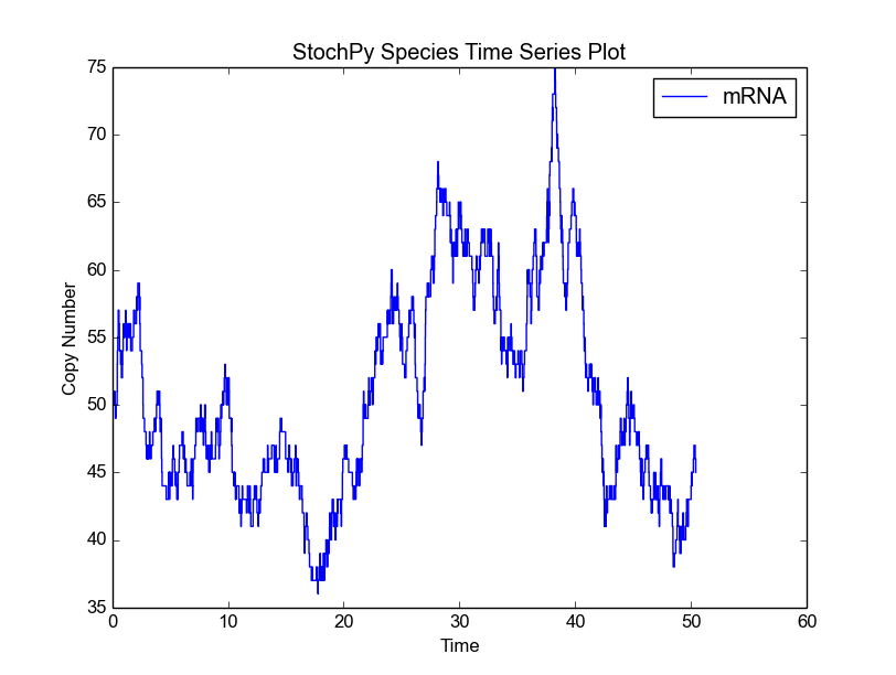
StochPy provides many example models, which can be used as a reference for building your own models. One of these examples is shown here:
# Reactions
R1:
    $pool > mRNA
    Ksyn

R2:
    mRNA > $pool
    Kdeg*mRNA

# Variable species
mRNA = 50.0

# Parameters
Ksyn = 10
Kdeg = 0.2
We call this the Immigration-death model which we use as the default model in StochPy. Here, we define two reactions: a zero-order reaction R1 synthesizing the species mRNA and a first-order reaction R1 degrading mRNA. Next, we set an initial mRNA copy number and finally the parameter values of the synthesis and degradation rate.
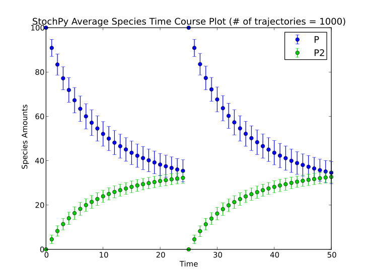
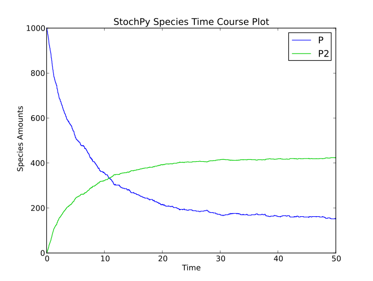
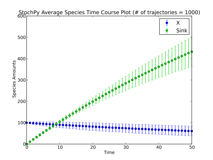
StochPy supports both time and species amount events (for more details see here). Here, we will illustrate these events with a model of dimerization of P to P2. The initial numbers of molecules of P and P2 are 100 and 0, respectively. We perform a stochastic simulation until t=50 for 1000 trajectories, which gives the following result.

We now add a time event where we reset the molecule numbers of P and P2 at t>=25. Events have access to the “current” simulation time using the _TIME_ symbol, which gives the following description of an event in the PySCeS MDL:
# Event definitions
Event: reset1, _TIME_ >= 25, 0.0
{
P2 = 0
P = 100
}
This event is incorporated in the dsmts-003-03.xml.psc file and simulation yields the following result:
>>> smod.Model('dsmts-003-03.xml.psc')
>>> smod.DoStochSim(end=50,mode='time',trajectories=1000)
>>> smod.GetRegularGrid()
>>> smod.PlotAverageSpeciesTimeSeries()
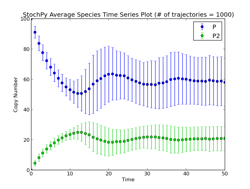
A second example is a species event where we reset the molecule numbers once molecule P is greater than 30:
# Event definitions
Event: reset2, P2 > 30, 0.0
{
P2 = 0
P = 100
}
This event is incorporated in the dsmts-003-04.xml.psc file and simulation yields the following result:
>>> smod.Model('dsmts-003-04.xml.psc')
>>> smod.DoStochSim(end=50,mode='time',trajectories=1000)
>>> smod.GetRegularGrid()
>>> smod.PlotAverageSpeciesTimeSeries()
So far, we used a time or species trigger but we can also combine both type of events:
# Event definitions
Event: reset3, P2 > 30 and _TIME_ > 20, 0.0
{
P2 = 0
P = 100
}
Species are now reset if P2 > 30 and if t>20. This event can also occur multiple times. Warning: do not use or specifications in event triggers, but use separate events instead. Finally, StochPy also allows for the mutation of parameters. Define this parameter as a fixed species (StochPy will give a warning that it does not occur in any reaction). This warning message is correct (it’s a parameter, not a species). Next, you can add a time event to modify the parameter during the simulation:
Event: jump1, _TIME_ >= 25, 0.0
{
k1 = 0.01
}
In this example, k1 is set to 0.01 at t=25 without any delay.
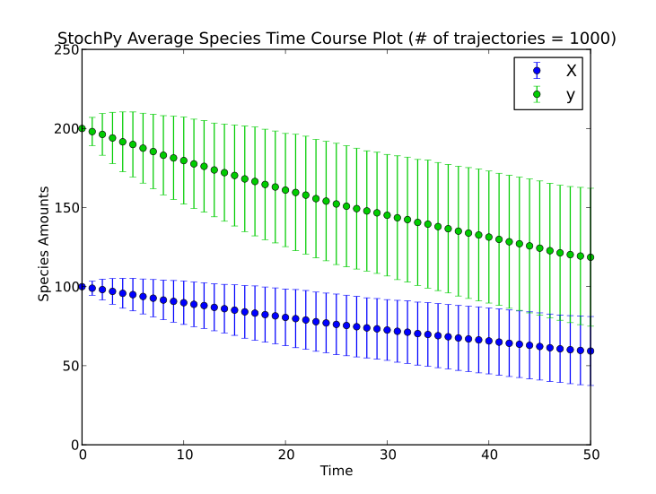
Here, we will shortly describe one example of an assignment rule for which we use a simple birth-death process of metabolite X. The assignment rules defines that a new species y = 2 * X:
# Assignment rules
!F y = 2.0*X
This assignment is incorporated in the dsmts-001-19.xml.psc file and simulation yields the following result.
The main module of this software package is the stochastic simulation algorithm module. In this module stochastic simulations and their analysis can be done. StochPy currently contains various Stochastic Simulation Algorithms (SSAs):
Use the following command to start to the SSA module:
>>> smod = stochpy.SSA()
Info: The Direct method is selected to perform the simulations
Parsing file: /home/user/Stochpy/pscmodels/ImmigrationDeath.psc
StochPy selects the direct method as default simulation algorithm and the immigration-death model as default stochastic model. As a result, you can use the high-level function DoStochSim() to run your first stochastic simulation:
>>> smod.DoStochSim()
Before we discuss doing these stochastic simulations in more detail, we first discuss some features of the SSA module. Upon initiation, it tries to load the interactive analysis environment. If successful, generated plots become immediately visible. Adding the optional argument IsInteractive = False ensures that no plots are shown after generation. This can be useful if the default behavior is undesired or if StochPy fails loading the interactive environment (e.g. on most computer clusters). In these cases, the generated plot can still be modified and saved to a file:
>>> smod = stochpy.SSA(IsInteractive=False)
>>> smod.DoStochSim()
>>> smod.PlotSpeciesTimeSeries()
>>> stochpy.plt.savefig(os.path.join(stochpy.output_dir,'example.png'))
The high-level function DoStochSim() accepts many arguments (e.g. method, trajectories, mode). Each of these settings are treated as “local” settings, i.e. they are forgotten if you perform a new stochastic simulation without these arguments. Alternatively, different high-level functions exist that allow for specifying “global” settings, i.e. they are used until you specify a new value or load a new model.
For instance, rather than using the method argument, the high-level function Method() can be used to select a simulation algorithm different than the default one:
>>> smod.Method('FirstReactionMethod')
Info: The First Reaction method is selected to perform the simulations
>>> smod.Method('NextReactionMethod')
Info: The Next Reaction method is selected to perform the simulations
>>> smod.Method('TauLeaping')
Info: The Explicit Tau-Leaping method is selected to perform the simulations
>>> smod.Method('Direct')
Info: The Direct method is selected to perform the simulations
Different strings can be provided to select e.g. the First Reaction Method. Currently, the valid case-insensitive keys are: ‘Direct’, ‘NextReactionMethod’ and ‘NRM’, ‘FirstReactionMethod’ and ‘FRM’, ‘Tauleaping’, ‘DelayedDirect’ and ‘Delayed’, ‘DelayedNRM’ and ‘DelayedNextReactionMethod’, ‘SingleMoleculeMethod’ and ‘SMM’, ‘FastSingleMoleculeMethod and ‘fSMM’.
The direct, next reaction method, and first reaction method are exact SSAs that suffer typically from extensive running times. We, therefore, also provide an inexact SSA: the tau-leaping method (click here). Additionally, we provide exact SSAs with delays (click here) and single molecule methods (here). As we will see shortly, different high-level functions must be used to run ‘standard’ SSAs, delayed SSAs, and SMM SSAs. Each of these high-level functions also accepts one of the supported methods as an argument.
As said, DoStochSim() also accepts the method argument:
>>> smod.DoStochSim(method='FRM')
The high-level function Model() can be used to select a model described in PySCeS MDL:
>>> smod.Model('BurstModel.psc')
Parsing file: /home/user/Stochpy/pscmodels/BurstModel.psc
>>> smod.Model(File='BurstModel.psc',dir='/home/user/Stochpy/pscmodels')
Parsing file: /home/user/Stochpy/pscmodels/BurstModel.psc
or in the systems biology markup language (SBML) if the appropriate dependencies are installed:
>>> smod.Model('dsmts-001-01.xml',smod.model_dir)
Info: extension is .xml
Info: single compartment model: locating "Death" in default compartment
Info: single compartment model: locating "Birth" in default compartment
Writing file: /home/user/Stochpy/pscmodels/dsmts-001-01.xml.psc

SBML2PSC
in : /home/user/dsmts-001-01.xml
out: /home/user/Stochpy/pscmodels/dsmts-001-01.xml.psc
Info: SBML data is converted into psc data
and is stored at: /home/user/Stochpy/pscmodels
Parsing file: /home/user/Stochpy/pscmodels/dsmts-001-01.xml.psc

>>> smod.model_file
'dsmts-001-01.xml.psc'
>>> smod.model_dir
'/home/user/Stochpy/pscmodels'
In this section, we illustrate performing stochastic simulations within StochPy in more detail. We can perform a simulation once we initialized the SSA module as shown in the previous section. We show it here once more:
>>> import stochpy
>>> smod = stochpy.SSA()
>>> smod.DoStochSim()
Info: 1 trajectory is generated
Number of time steps 1000  End time  15.2161060754
Simulation time 0.0805060863495
By default StochPy generates one trajectory of 1000 time steps. StochPy can do simulations for a user-specified number of time steps:
>>> smod.Timesteps(10**5)
or until a certain simulation end time:
>>> smod.Endtime(100)
In this example, we set the simulation end time to 100. Be careful if you specify a certain end time because the reactions in the model determine when a certain reaction fires. So, dT—the time between two reactions to fire—is large if the majority of the reactions is unlikely to fire, but becomes small if the majority of the reactions is very likely to fire. As a result, model A could take for instance 1000 time steps to reach the user specified end time, but model B could take more than 1000000 time steps to reach the user specified end time.
The high-level function DoStochSim() accepts the arguments: method, mode, end, trajectories, IsTrackPropensities, species_selection, IsOnlyLastTimepoint. Hence, stochastic simulations in StochPy can be done with one high-level function:
>>> smod.DoStochSim(method = 'direct', mode = 'time', end = 50)
Info: The Direct method is selected to perform the simulations
Parsing file: /home/user/Stochpy/pscmodels/ImmigrationDeath.psc
Info: 1 trajectory is generated
Number of time steps 3807  End time  50
Simulation time 0.142936944962
Remember that settings provided as arguments in this function are “local” rather than “global”:
>>> smod.Trajectories(5)
>>> smod.DoStochSim()
Info: 5 trajectories is generated
simulation done!
Info: Time simulation output of the trajectories is stored at ...
Info: output is written to: /home/user/Stochpy/ssa_smod.log
Simulation time 0.345077991486
>>> smod.DoStochSim(trajectories=10)
Info: 10 trajectories are generated
Info: Time simulation output of the trajectories is stored at ...
Info: output is written to: /home/user/Stochpy/ssa_smod.log
Simulation time 0.48316593202
>>> smod.DoStochSim()
Info: 1 trajectory is generated
simulation done!
Info: Number of time steps 1000 End time 49.1597126518
Info: Simulation time 0.07931
In this example, we globally set the number of trajectories to 5. Then, we run DoStochSim() with trajectories=10 as additional argument, hence we generate 10 trajectories. Finally, we run DoStochSim() without additional arguments. Because we used the argument trajectories before in DoStochSim(), we now reset the number of trajectories to the default value.
Importantly, the high-level function DoStochSim() supports only the simulation of the traditional SSAs. Different high-level functions are necessary for the simulation of e.g. delayed SSAs. For example, DoStochSim() will switch back to the direct method if e.g. the delayed direct method is provided:
>>> smod.DoStochSim(method='DelayedDirect')
Info: Delayed Direct Method is selected.
Parsing file: /home/timo/Stochpy/pscmodels/ImmigrationDeath.psc
Info: No reagents have been fixed
*** WARNING ***: (DelayedDirectMethod) was selected. Switching to the normal Direct Method.
Info: Direct method is selected to perform stochastic simulations.
Additionally, StochPy can modify both parameter values and initial species amounts with the following high-level functions:
>>> smod.ChangeParameter('Ksyn',5)
>>> smod.ChangeInitialSpeciesAmount('mRNA',100)
Note that both ChangeParameter() and ChangeInitialSpeciesAmount() change parameter values and species amounts, respectively, in the current StochPy object. In other words, no changes are made to the model source file and made changes are lost after loading a different model. Alternatively, simply adjust the model description file (in the directory where the model is stored) and reload the model with the following high-level function:
>>> smod.Reload()
Parsing file: /home/user/Stochpy/pscmodels/ImmigrationDeath.psc
We understand that during an interactive session, it can become difficult to remember all specified settings. Therefore, we provide high-level functions that provide a summary of the status of the current settings:
>>> smod.ShowSpecies()
['mRNA']
>>> smod.ShowOverview()
Current Model:        ImmigrationDeath.psc
Number of time steps: 1000
Current Algorithm:    <class 'stochpy.DirectMethod.DirectMethod'>
Number of trajectories:       1
Propensities are not tracked
Here, ShowSpecies() gives a list of all the species in the model and ShowOverview() gives all the current settings. Note that it is also possible to save an interactive session to a Python script:
>>> stochpy.SaveInteractiveSession("interactiveSession1.py")
Next, one can simply reload interactive session by starting this script in iPython:
$ ipython interactiveSession1.py
Or by running it inside iPython (make sure you are in the correct working directory):
>>> run interactiveSession1.py
StochPy returns the “raw” stochastic simulation output, i.e. for each firing time we store the copy number of each species and if desired also the propensity of each reaction. This can result in memory issues for models with many species (and reactions). For this reason, StochPy provides several ways to reduce the amount of stored data. We provide two arguments: species_selection and rate_selection which can be used to specify for which species and rates we store its copy number and propensity at each firing time. By default, we store this information for each species and for none of the rates. Adding IsTrackPropensities = True as argument results in storing this information for every rate. Here, we provide an example of a model that consists of 50 species and 98 reactions. We store two species and the propensities of two reactions.
>>> smod.Trajectories(1)
>>> smod.Model('chain50.psc')
>>> smod.DoStochSim(species_selection = ['S1','S5'],rate_selection=['R1','R15'])
>>> smod.data_stochsim.species_labels
 ['S1', 'S5']
>>> smod.data_stochsim.species
array([[ 1.,  0.],
    [ 0.,  0.],
    [ 0.,  0.],
    ...,
    [ 0.,  0.],
    [ 0.,  0.],
    [ 0.,  0.]])
>>>  smod.data_stochsim.propensities
array([[ 1.,  0.],
    [ 0.,  0.],
    [ 0.,  0.],
    ...,
    [ 0.,  0.],
    [ 0.,  0.],
    [ 0.,  0.]])
>>>  smod.data_stochsim.propensities_labels
 ['R1', 'R15']
In addition, the boolean IsOnlyLastTimepoint can be exploited if users are only interested in species amounts after a specific time. Note that if IsOnlyLastTimepoint = True, many functionalities such as plotting and determining statistics are disabled.
>>> smod.Model('ImmigrationDeath.psc')
>>> smod.DoStochSim(end=50,mode='time',IsOnlyLastTimepoint = True)
>>> smod.data_stochsim.species # species amounts at the last time point (t=50)
    array([[55.]])
>>> smod.data_stochsim.time # stored time points (t=50)
    array([[50.]])
Before we discuss the plotting features of StochPy, we first want to discuss some potential issues. StochPy exploits Matplotlib for plotting. If Windows is your operating systems, interactive plotting with Matplotlib can result in figure freezing. If you encounter figure freezing, we suggest to try out different back-ends (http://matplotlib.org/faq/usage_faq.html#what-is-a-backend). TkAgg is probably the best for interactive plotting, but is not available on every operating system and/or python environment:
>>> stochpy.plt.switch_backend('TkAgg')
Alternatively, different non-interactive back-ends are available. An example of this is the ‘Agg’-backend:
>>> stochpy.plt.switch_backend('Agg')
>>> smod.DoStochSim()
>>> smod.PlotSpeciesTimeSeries() # no plot is shown
>>> stochpy.plt.savefig(stochpy.os.path.join(stochpy.output_dir,'test1.png')
If you switch to a non-interactive back-end, make sure to initialize the SSA object with IsInteractive= False:
>>> smod = stochpy.SSA(IsInteractive=False)
>>> smod.DoStochSim()
>>> smod.PlotSpeciesTimeSeries()
>>> stochpy.plt.savefig(stochpy.os.path.join(stochpy.output_dir,'test1.png')
>>> cmod = stochpy.CellDivision(IsInteractive=False)
Plotting in Windows:
StochPy provides many preprogrammed analysis techniques that can be exploited to analyze done stochastic simulations. Here, we will start with a discrete time series plot:
>>> smod.PlotSpeciesTimeSeries()
This function accepts many arguments of which species to plot and mark-up details are examples:
>>> smod.PlotSpeciesTimeSeries(linestyle='dashed',linewidth=2,xlabel='Time (s)')
By default, StochPy creates a figure legend. This legend can be (i) turned off with IsLegend = False or (ii) moved to a different location with legend_location. The default legend location is the upper right corner. Both IsLegend and legend_location are arguments of each plotting function.
Plots are directly shown if the interactive environment is successfully loaded. On Windows, interactive plotting in Python can cause figures to freeze. If you encounter this issue, please have a look at this section (changing the Matplotlib backend solves typically the problem). It is also possible to turn off the interactive plotting feature:
>>> smod = stochpy.SSA(IsInteractive = False)
With the interactive modes turned off, plotting is still possible but the figures are not directly shown. The first command shows the figure (if possible) and the second command saves it to a (pdf) file:
>>> stochpy.plt.show()
>>> stochpy.plt.savefig('myfigure.pdf')
The second analysis feature offered by StochPy is determining both the mean and standard deviation of each species in the simulated model:
>>> smod.PrintSpeciesMeans()
Species       Mean
mRNA  49.969
>>> smod.PrintSpeciesStandardDeviations()
Species       Standard Deviation
mRNA  7.104
Calculating the mean and standard deviation of each species in a stochastic simulation is not as straightforward as it may sound. The time between two events is not constant, thus it is necessary to track the time spent in each state for each species. These species statistics can also be accessed via the data_stochsim model object as Python dictionaries:
>>> smod.data_stochsim.species_means
{'mRNA': 49.9689958686}
>>> smod.data_stochsim.species_standard_deviations
{'mRNA': 7.1044044211 }
Also, StochPy allows the calculation and analysis of event waiting times. Event waiting times are the times between two subsequent firings of a particular reaction. StochPy can offer this unique feature, because StochPy returns all events. See the Examples section for a plot of an event waiting times distribution.
>>> smod.GetWaitingtimes()
>>> smod.PlotWaitingtimesDistributions()
>>> smod.PrintWaitingtimesMeans()
Furthermore, StochPy can determine propensities at each time point during the simulation. Propensities data is not stored by default. The boolean argument IsTrackPropensities of the high-level function DoStochSim() must be set to True:
>>> smod.DoStochSim(IsTrackPropensities=True)
>>> smod.PlotPropensitiesTimeSeries()
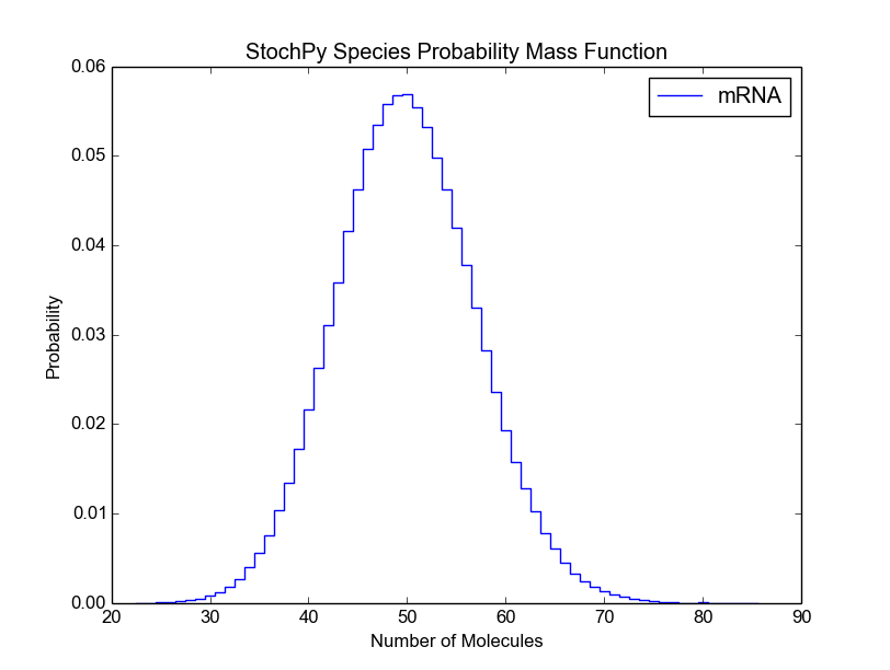
This means that we can generate two types of time series data: species and propensities. For both of these data types, probability distributions can be generated:
>>> smod.PlotPropensitiesDistributions()
>>> smod.PlotSpeciesDistributions()
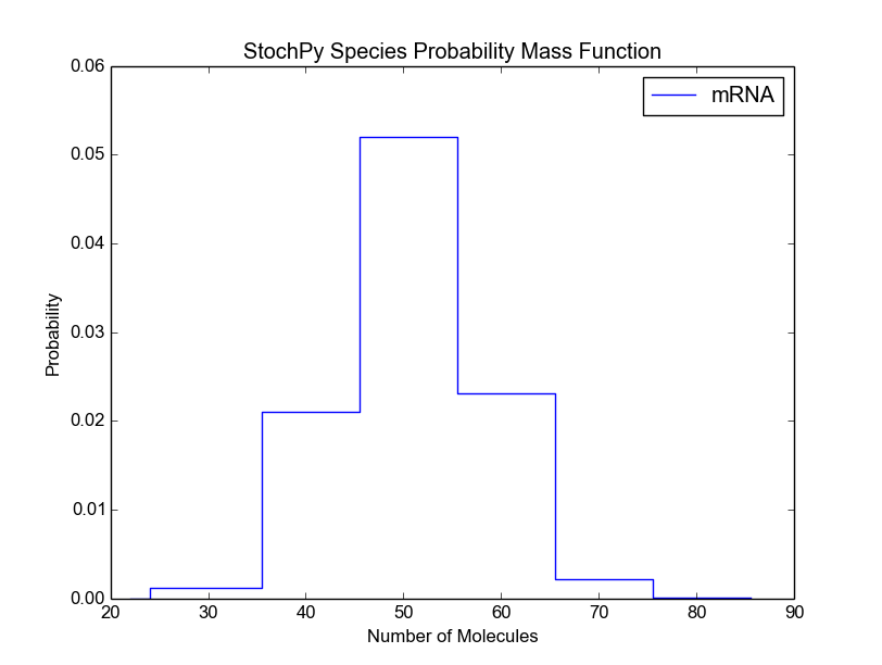
Again, both functions accept many different arguments (see smod.PlotSpeciesDistributions?). For example, we can modify the bin size of the species probability density function:
>>> smod.DoStochSim(end=10**6,mode='steps')
>>> smod.PlotSpeciesDistributions()
>>> smod.PlotSpeciesDistributions(bin_size=10)
Before we continue with the remaining preprogrammed analysis techniques, we want to briefly discuss a general problem of stochastic simulations. For a certain kind of analysis method, it is typically difficult to determine beforehand the right number of time steps. Therefore, StochPy provides a function, DoCompleteStochSim(), which continues until the first four moments converge within a user-specified error (default = 0.001).
>>> smod.DoCompleteStochSim(error=0.001)
>>> smod.PrintSpeciesMeans()
>>> smod.PrintSpeciesStandardDeviations()
>>> smod.PlotSpeciesDistributions()
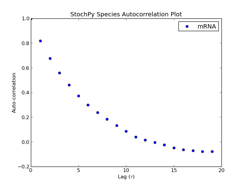
The Gillespie algorithms generate data at irregular time points. However, StochPy also offers an approach which returns data on a fixed regular time grid. A grid of which the user can specify the resolution (n_samples). The formation of such a regular grid allows for the analysis of autocorrelation (and autocovariance) of species and/or propensities within StochPy. Autocorrelation is the cross-correlation, a measure of similarity of a signal with itself. For different time separations (lags), this similarity can be determined which results a value between 1 and -1. Here, 1 corresponds to positive correlation and -1 to negative correlation. Typically, the first 50 lags are of interest. Here, we show the first 20 lags:
>>> smod.Model('ImmigrationDeath.psc')
>>> smod.DoStochSim(trajectories=1,end=1000,mode='time',
    IsTrackPropensities=True)
>>> smod.GetSpeciesAutocorrelations(gridpoints=1001)
>>> smod.PlotSpeciesAutocorrelations(nlags=20)
>>> smod.GetPropensitiesAutocorrelations()
>>> smod.PlotPropensitiesAutocorrelations(nlags=20)
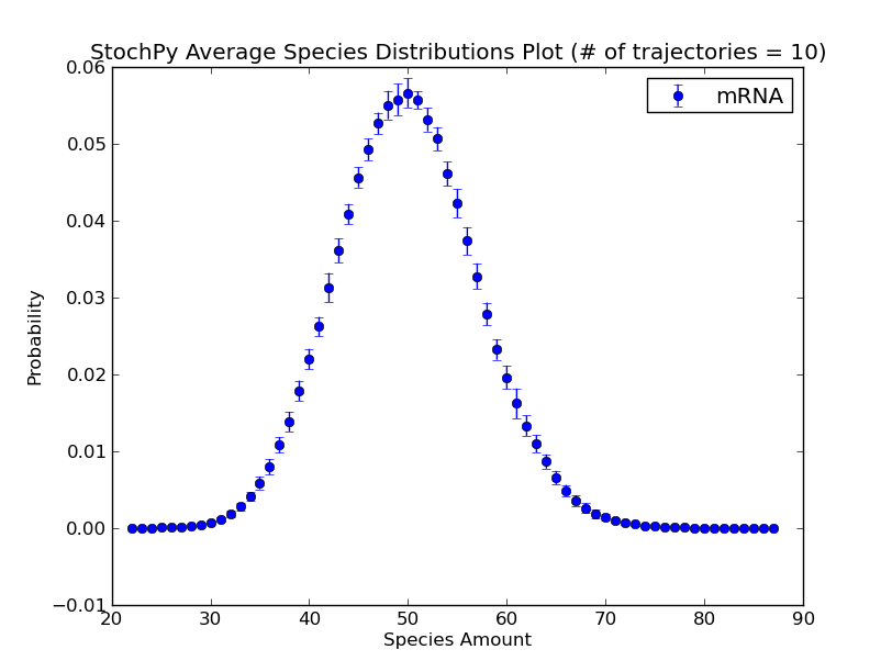
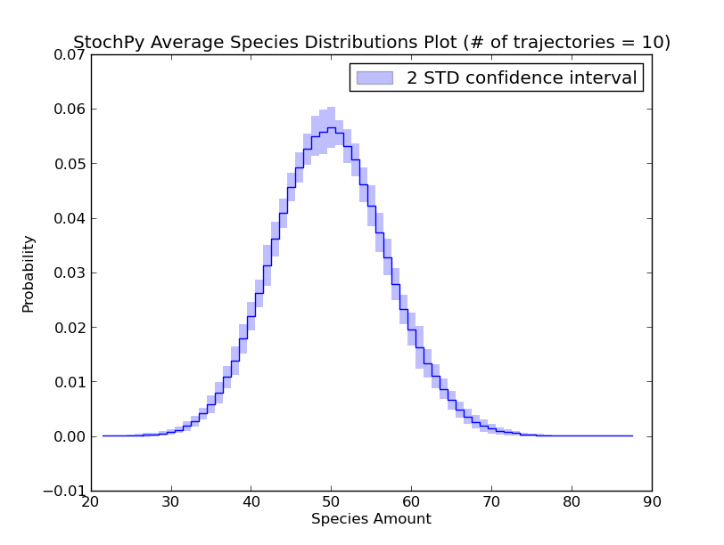
Additionally, we can exploit the formation of a regular grid for analyzing multiple generated trajectories. Via StochPy, we can generate e.g. average time series plots for both species and propensities. Here, we discuss two different plotting functionalities for analyzing probability distributions of species averaged over multiple trajectories. The argument nstd can be used to set the number of standard deviations of the error bars:
>>> smod.DoStochSim(trajectories=10,end=10**5)
>>> smod.GetRegularGrid(n_samples=51)
>>> smod.PlotAverageSpeciesDistributions()
>>> smod.PlotAverageSpeciesDistributionsConfidenceIntervals(nstd=2)
We already explained that we do not have to store the species amounts of every species. As a consequence, we can only plot data for “stored” species. Additionally, we can use the high-level plotting functions to plot a subset of the stored data:
>>> smod.PlotSpeciesTimeSeries(species2plot = ['S1','S2'])
>>> smod.PlotPropensitiesTimeSeries(rates2plot = 'R1')
>>> smod.PlotWaitingtimesDistributions(rates2plot = 'R2')
>>> smod.PlotSpeciesDistributions('S4')
AssertionError: Species S4 is not in the model
StochPy also offers stochpy.plt (a renamed version of matplotlib.pyplot) to manipulate generated plots or to generate your own plots:
>>> smod.PlotSpeciesTimeSeries(marker = 'v')
>>> stochpy.plt.title('Your own title')
>>> stochpy.plt.xlabel('Time (s)')
>>> stochpy.plt.xlim([0,10**3])
>>> stochpy.plt.savefig('stochpy_plot.pdf')
Besides plotting features StochPy allows printing and exporting of generated data sets. Printing data is only useful for small datasets, so we prefer using Export2File() which allows data storage in a text file for e.g. external manipulation:
>>> smod.Export2File()
>>> smod.Export2File(analysis='timeseries',datatype='species')
>>> smod.Export2File(analysis='timeseries',datatype='propensities')
>>> smod.Export2File(analysis='distributions',datatype='species')
>>> smod.Export2File(analysis='distributions',datatype='waitingtimes')
>>> smod.Export2File(analysis='distributions',datatype='autocorrelations')
>>> smod.Export2File(analysis='timeseries',datatype='species',IsAverage=True)
StochPy also supports the import of previously exported time series data:
>>> smod.Import2StochPy('myfile','myfiledir',delimiter='\t')
Finally, one can access and manipulate data objects that store the simulation data to perform your own type of analysis in StochPy. See Using Stochpy as a Library.
Here, we use the ‘decaying-dimerizing’ model to illustrate the potential advantage of inexact SSA solvers. While exact solvers always simulate one reaction per time step, inexact solvers such as the tau-leaping method try to simulate more than one reaction per time step. They do this by asking the following question: How often does each reaction fire in the next specified time interval tau. The larger the value of this tau the more reactions can fire within this time period, but this tau value must be small enough to make sure that no propensity function suffers from a significant change.
As a result, a significant speed advantage can be obtained for models where molecules are present in large quantities. An example of such a system is the decaying-dimerizing model, where S1(t=0)= 100000. Next, we simulate this model with first the tau-leaping and secondly the direct method of which the results are shown below. Note that information about exact firing times (and therefore also event waiting times) cannot be obtained with this tau-leaping method:
>>> smod.Model('DecayingDimerizing.psc')
>>> smod.DoStochSim(method='TauLeaping',end=50,mode='time')
>>> smod.PlotSpeciesTimeSeries()
>>> smod.DoStochSim(method='Direct',end=50,mode='time')
>>> smod.PlotSpeciesTimeSeries()
>>> stochpy.plt.xscale('log')

Tau-leaping methods exploit a error-control parameter, epsilon, that bounds the expected change in the propensity functions. This epsilon value ranges between 0-1 where smaller values result in more accurate simulations (but also a smaller tau size and longer simulations). We set this value, by default, to 0.03 (as is also done by Cao et al. 2006). For the decaying-dimerizing model, the tau-leaping method is about 50 times faster than the direct method. StochPy allows users to manipulate this setting with the argument epsilon, as we will show next.
We now set it to 0.05:
>>> smod.DoStochSim(method='TauLeaping',end=50,mode='time',epsilon = 0.05)
The tau-leaping method is now about 100 times faster than the direct method. Be careful with too large values of epsilon, because this will eventually result in incorrect simulation results. Therefore, we advice users of the tau-leaping method to verify the outcome against that of an exact solver. A more strict value can be necessary if you want an accurate prediction of species quantities at different time points. An example is the dsmts-001-05 model of the test suite from Evans et al. 2008. We wanted an accurate prediction at t=0,1, ... 50 for which an epsilon value of 0.01 was required.
* Warning *
The tau-leaping method automatically reduces the epsilon value for second and third-order reactions. StochPy, therefore, tries to tries to determine the order of each reaction, the “highest order of reaction” (HOR) for each species and its contribution. This works properly for mass-action kinetics, but is likely to fail for non mass-action kinetics. Use the following commands to access the automatically generated results of StochPy
>>> smod.Model('DecayingDimerizing.psc')
>>> smod.Method('TauLeaping')
>>> smod.SSA.parse.reaction_orders
[1,2,1,1]
>>> smod.SSA.parse.species_HORs
[2,1,0]
>>> smod.SSA.parse.species_max_influence
[2,1,0]
These results are correct (the model is also described by mass-action kinetics). All reactions are first order, except the second reaction. This is a dimerization reaction of species S1. Therefore, the highest order of reaction (HOR) of S1 is 2. Species S2 acts as reactant in a first-order reaction (HOR, S2 = 1) and S3 is not a reactant (HOR, S3 = 0). Finally, species_max_influence gives the highest contribution of a species to its HOR.
StochPy allows users to modify the three lists shown above directly, but one can also provide them as arguments to the DoStochSim() function:
>>> smod.DoStochSim(end=50,mode='time',method='TauLeaping',reaction_orders = [1,2,1,1],
                    species_HORs = [2,1,0], species_max_influence = [2,1,0])
Finally, StochPy’s implementation of the tau-leaping method defines ‘critical reactions’, i.e. reactions that are within a few firings of exhausting (one of) its reactants. These critical reactions are used to reduce the probability for a negative population by allowing these reactions to fire only once per time step. The automated determination of critical reactions works fine for most rate equations, but could go wrong for some very specific rate equations. We, therefore, allow you to specify reaction(s) that can fire no more than once during a single time step for the entire simulation. While it is not necessary for the decaying-dimerizing model, we now set R4 as a critical reaction for the entire simulation:
>>> smod.DoStochSim(end=50,mode='time',method='TauLeaping',critical_reactions = ['R4'])
Because it is not necessary for this model, the simulation time will increase notably (only 5 times faster than the direct method).
Delayed stochastic algorithm extent the Gillespie stochastic simulation algorithm (SSA) to a system with delays. A delayed reaction consists of an exponential waiting time as initiation step with a subsequent delay time. We implemented both the Delayed Direct Method (Cai 2007, J. Chem. Phys) and the Delayed Next Reaction Method (Anderson 2007, J. Chem. Phys).
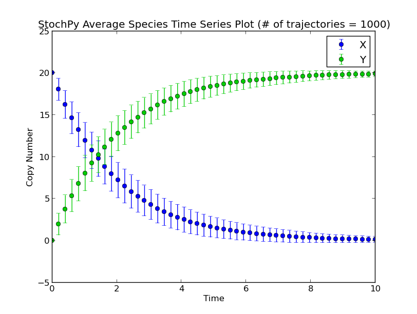
Before we perform a delayed stochastic simulation, we first perform a normal stochastic simulation with a simple model where X molecules are converted to Y molecules:
>>> smod.Model('Isomerization.psc')
>>> smod.DoStochSim(mode='time',end=10,trajectories=1000)
>>> smod.GetRegularGrid(n_samples=50)
>>> smod.PlotAverageSpeciesTimeSeries()
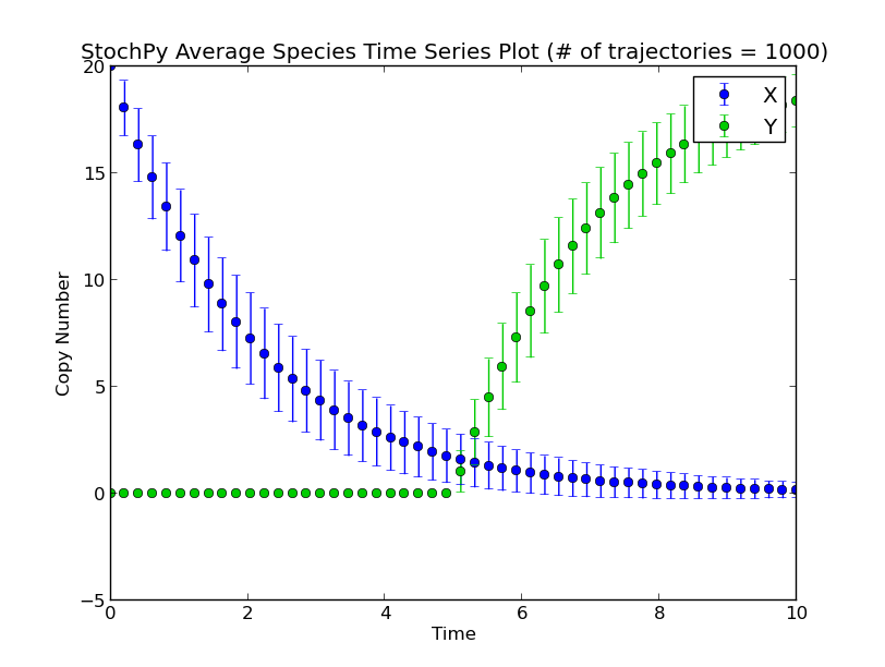
Next, we set a fixed delay of 5 seconds on reaction R1. This means that after R1 fires, a X molecule is consumed and it takes exactly 5 seconds before a Y molecule is produced:
>>> smod.SetDelayParameters({'R1':('fixed',5)})
>>> smod.DoDelayedStochSim(mode='time',end=10,trajectories=1000)
>>> smod.GetRegularGrid(n_samples=50)
>>> smod.PlotAverageSpeciesTimeSeries()
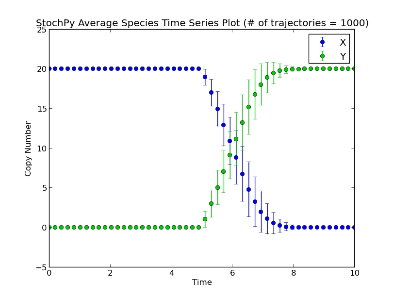
There exist two types of delayed reactions: consuming and nonconsuming delayed reactions. For consuming delayed reactions, the reactants are consumed at initiation and for nonconsuming delayed reactions, the reactants are consumed at completion. In both cases, the products are updated at completion. By default, delayed reactions are “consuming delayed reactions”. Alternatively, we can simulate nonconsuming delay reactions. In this example, after reaction R1 fires, it takes exactly 5 seconds before a particular X is degraded and a particular Y is produced:
>>> smod.SetDelayParameters({'R1':('fixed',5)},nonconsuming_reactions=['R1'])
>>> smod.DoDelayedStochSim(mode='time',end=10,trajectories=1000)
>>> smod.GetRegularGrid(n_samples=50)
>>> smod.PlotAverageSpeciesTimeSeries()
Note that performing a delayed stochastic simulation is not allowed without setting delayed parameters:
>>> smod.Model('ImmigrationDeath.psc')
Info: Please mind that the delay parameters have to be set again.
Parsing file: /home/timo/Stochpy/pscmodels/ImmigrationDeath.psc
Info: No reagents have been fixed
>>> smod.DoDelayedStochSim()
AttributeError: No delay parameters have been set.
Please first use the function .SetDelayParameters().
An empty set of delayed parameters is sufficient, but realize that this is similar to doing a non-delayed stochastic simulation:
>>> smod.SetDelayParameters({})
>>> smod.DoDelayedStochSim()
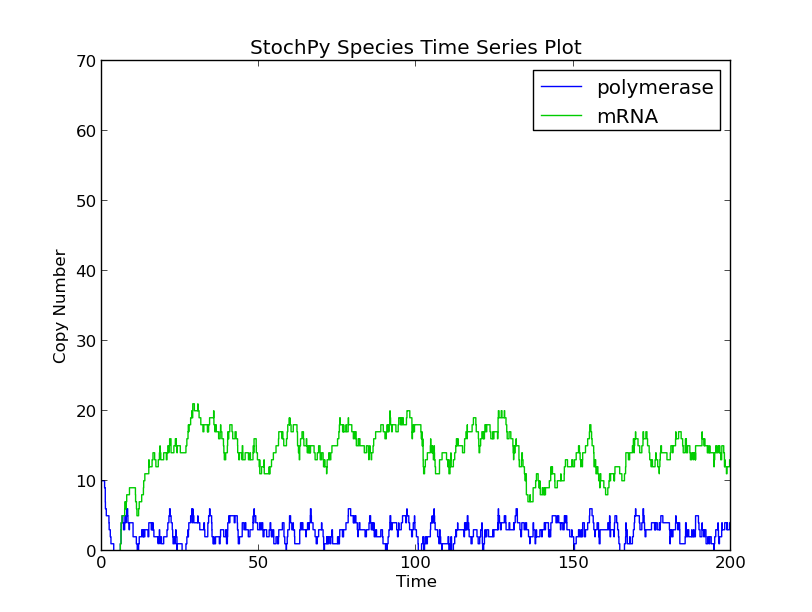
Here, we use a small model of gene transcription to illustrate the difference between consuming and nonconsuming delayed reactions. RNA polymerase can bind to the promoter region of a gene, which starts the transcription process. When the RNA polymerase leaves the promoter region and elongation phase of the transcription process starts, a next RNA polymerase can bind to the gene. This means that, if we assume that the number of RNA polymerases is relatively large, gene transcription can be viewed as a nonconsuming reaction.
Modeling this process as a nonconsuming reactions gives completely different results as is shown here with two simple simulations. First, we simulated this process as a consuming reaction. The available RNA polymerase pool depletes quickly which reduces the formation rate of mRNA chains:
>>> smod.Model('Polymerase.psc')
>>> smod.Endtime(200)

>>> smod.SetDelayParameters({'R1':('fixed',5)})
>>> smod.DoDelayedStochSim()
>>> smod.PlotSpeciesTimeSeries()
>>> stochpy.plt.ylim(0,70)
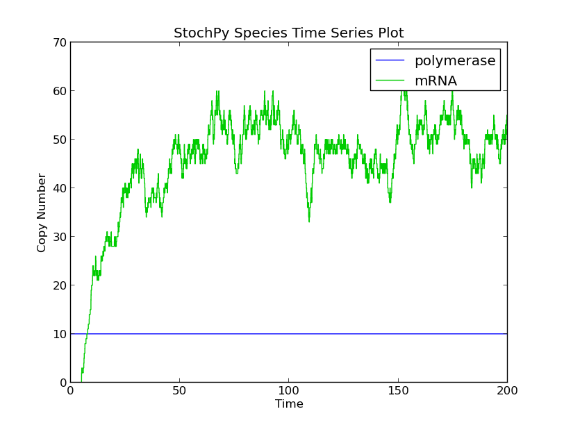
Secondly, we modeled this process as a nonconsuming reaction. As a result, the available RNA polymerase stayed constant, and therefore, significantly more mRNA chains were produced.
>>> smod.SetDelayParameters({'R1':('fixed',5)}, nonconsuming_reactions = 'R1')
>>> smod.DoDelayedStochSim()
>>> smod.PlotSpeciesTimeSeries()
>>> stochpy.plt.ylim(0,70)
In stochastic simulations, reaction times are exponential random variables with mean and standard deviation 1/a0; a0 is the sum of all propensities. For certain processes, reaction times can be distributed differently (think of e.g. lumped reactions). One way to circumvent this is to exploit delays. We developed a method called the Single Molecule Method (SMM) that approaches reactions differently. Here, both the exponential step and a potential delay are replaced by a reaction time for the whole reaction. More importantly, the reaction time does not have to be drawn from an exponential distribution, whereas can be drawn from any distribution.
The propensity is typically a rate parameter multiplied with one or more species. For example, for the first-order reaction X -> Y, the propensity function is k1*X. Hence, the mean reaction time decreases with increasing X and vice versa. The SMM treats the copy number differently: Putative reaction times are determined for each set of substrate molecules individually. This means that, for our example model X -> Y, we determine a putative reaction time for each X molecule. These putative reactions times can be fixed or drawn from a distribution of choice. Of course, negative values are not allowed so be careful with e.g. normal distributions. If a molecule acts as a reactant in multiple reactions, it has a putative reaction time for each of these reactions. The shortest putative reaction time will ‘win’ and the molecule will react in this reaction channel. This is similar to the Next Reaction Method developed by Gibson and Bruck, with the difference that we look at single molecule rather than single reactions.
Note that the SMM can be rather slow, especially for models with many second-order reactions with high reactant copy numbers. For second-order reactions, every combination of molecules should be considered. We use a simple example to illustrate this. Consider the reaction A + B > C, with ten molecules of A and hundred molecules of B. There are in total thousand different reactions possible, i.e. each molecule of A can react with hundred different molecules of species B. For each of these thousand reactions, a putative reaction time is generated. After selecting the reaction with the shortest putative reaction time, many modifications have to be made to the system. For instance, all reactions that belong to the selected A and B molecules have to be deleted. Imagine what happens if multiple reactions can use these compounds as reactants.
Often, the majority of reactions in a model are regular exponential reactions. We, therefore developed the fast Single Molecule Method (fSMM) to speed-up the SMM simulation time. This method combines a regular Next Reaction Method and the SMM. The main advantage is that only reactions which are given a particular putative reaction time distribution, the single molecule reactions, are treated as in the SMM. The other reactions have a exponential putative time distribution and are simulated as in a normal Next Reaction Method. Hence, the number of putative reaction times stored will be significantly decreased, resulting in a faster search for the shortest putative reaction time.
Before we use a simple example to illustrate the single molecule method, we first discuss a few important points:
In this first example model, we explicitly model a intermediate form of the polymerase, polymerase moving. After exactly 60 seconds, the moving polymerase produces mRNA and is free again.
>>> smod.Model('TranscriptionIntermediate.psc')
>>> smod.SetPutativeReactionTimes({'R2':('fixed',60)})
>>> smod.DoSingleMoleculeStochSim(method = 'fSMM')
>>> smod.PlotSpeciesTimeSeries()
>>> smod.PlotWaitingtimesDistributions()
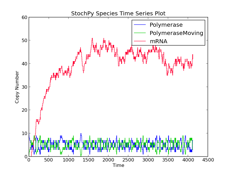
Interestingly, the waiting times between subsequent firings of R1 and R2 match; R2 fires exactly 60 time units after R1 fires. Note that in a delayed-SSA, the intermediate form is not modeled explicitly.
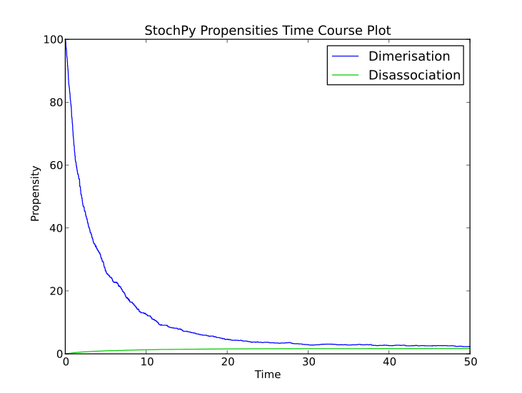
Stochastic simulations are done with a dimerization model to illustrate how you can use the stochastic simulation algorithm module. This model contains two species, denoted by P and P2:
>>> import stochpy
>>> smod = stochpy.SSA()
>>> smod.Model('dsmts-003-02.xml.psc')
>>> smod.DoStochSim(end = 50,mode = 'time',IsTrackPropensities=True)
Info: 1 trajectory is generated
Number of time steps 575  End time  50
Simulation time: 0.0349988937378

>>> smod.PlotSpeciesTimeSeries()
>>> smod.PlotPropensitiesTimeSeries()
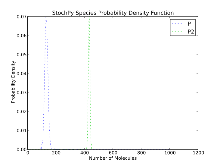
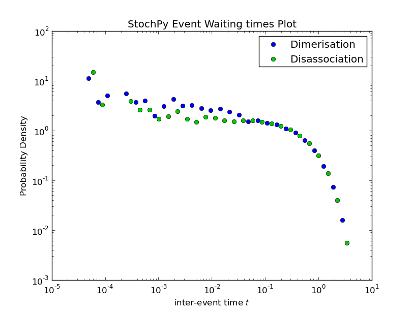
Doing a simulation for more time steps for allows the calculation of more accurate species distributions and event waiting time distributions:
>>> smod.DoStochSim(end=5000,mode = 'time',IsTrackPropensities=True)
Info: 1 trajectory is generated
Number of time steps 17799  End time  5000
Simulation time 1.39394283295
>>> smod.PlotSpeciesDistributions()
>>> smod.PlotWaitingtimesDistributions()
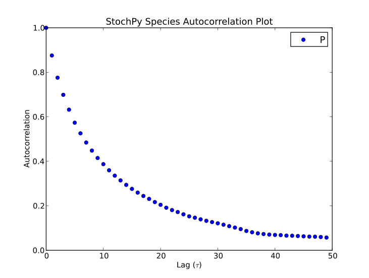
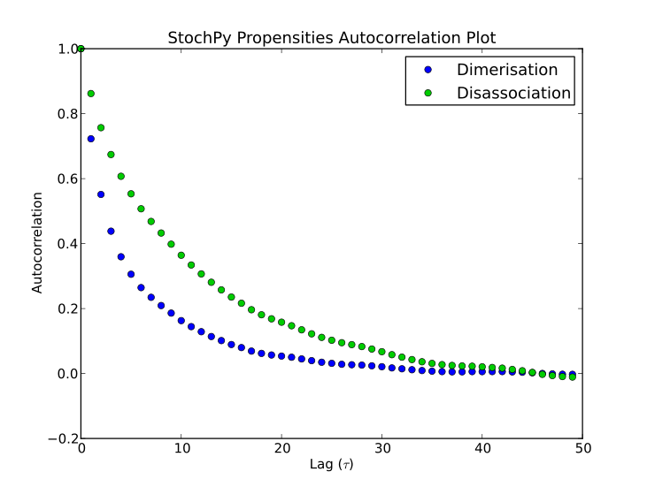
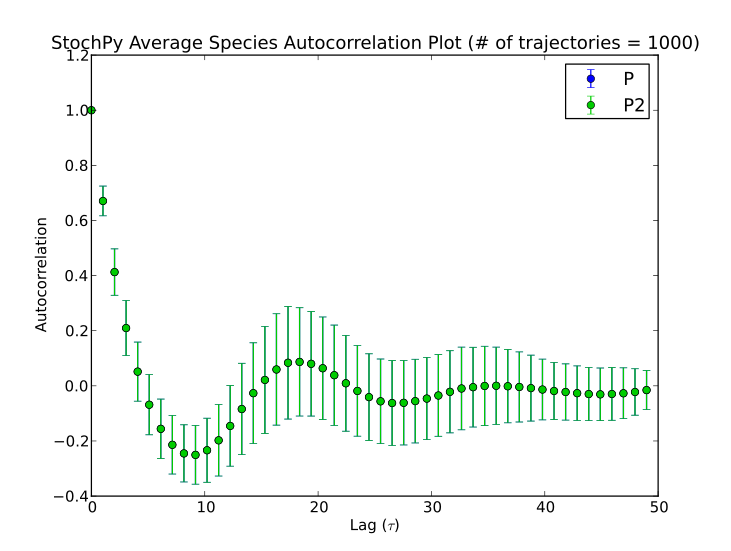
Finally, autocorrelations for both species and propensities can be determined:
>>> smod.GetSpeciesAutocorrelations()
>>> smod.GetPropensitiesAutocorrelations()
>>> smod.PlotSpeciesAutocorrelations(species2plot='P',nlags=50)
>>> smod.PlotPropensitiesAutocorrelations(nlags=50)
StochPy is written in Python, so users of StochPy can take advantage of e.g. the scientific libraries that are available in Python. We illustrate this here with the immigration-death model. This immigration-death model contains one species, mRNA. mRNA is synthesized with a constant rate and degraded with a first-order reaction. The immigration-death model is one of the simplest examples of a Poisson process: A stochastic process where events occur continuously and independently of one another.
One of the characteristics of a Poisson process is that the mean and variance are identical. In this example, we use a synthesis rate of 10 and a degradation rate of 0.2, thus both the mean and variance are 50. Here, we will first draw N samples from a Poisson distribution with mean = 50. Secondly, we perform a stochastic simulation for N time steps. The initial mRNA copy number is 50. After the simulation, we create a probability density function of the done stochastic simulation. Finally, we create a histogram of the randomly generated Poisson data and add this to the existing plot of the mRNA probability density function. If N is large enough (we use N = 2.5 million), both distributions will be almost identical.
>>> import numpy as np
>>> lambda_ = 50
>>> N = 2500000
>>> data = np.random.poisson(lambda_,N)
>>> smod.Model('ImmigrationDeath.psc') # Ksyn=10, Kdeg=0.2, and mRNA(init)=50
>>> smod.DoStochSim(end=N,mode='steps')
>>> smod.PlotSpeciesDistributions(linestyle= 'solid')
>>> n, bins, patches = stochpy.plt.hist(data-0.5, max(data)-min(data),
    normed=1, facecolor='green')
>>> smod.PrintSpeciesMeans()
mRNA  49.912
>>> smod.PrintSpeciesStandardDeviations()
Species       Standard Deviation
mRNA  7.073

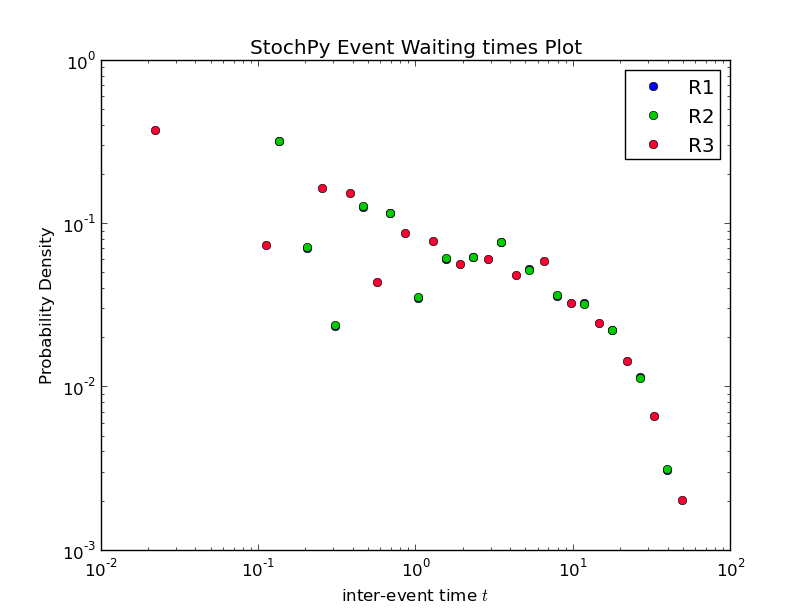
In the next example, we use a model that describes stochastic mRNA synthesis by a switching gene. The product mRNA is synthesized only when the switching gene is the ON state. We will compare two kinetic parameter settings leading to a bursty and a non-bursty mode of transcription. For both parameter settings, we will perform a stochastic simulation of 1.5 million time steps and subsequently create (i) a probability distribution of the mRNA copy numbers and (ii) a probability distribution of the mRNA synthesis event waiting times. We also know the analytical solutions, and we will add them to both plots. Finally, we demonstrate how we can manipulate the generated plots.
We will observe completely different distributions of the mRNA copy number. More specifically, we get a bimodal and a unimodal distribution of mRNA copy number for the first and second set of parameter values, respectively:
>>> import numpy as np
>>> import mpmath
>>> import stochpy
>>> mpmath.mp.pretty = True

>>> def GetAnalyticalPDF(kon,koff,kdeg,ksyn):
    """ Get the analytical probability density function.
    The analytical solution is taken from Sharezaei and Swain 2008 -
    Analytical distributions for stochastic gene expression """
    import mpmath
    mpmath.mp.pretty = True
    x_values = np.linspace(0,50,10000)
    y_values = []
    for m in x_values:
        a = ((ksyn/kdeg)**m)*np.exp(-ksyn/kdeg)/mpmath.factorial(m)
        b = mpmath.mp.gamma((kon/kdeg)+m)*mpmath.mp.gamma(kon/kdeg+koff/kdeg)\
        / (mpmath.mp.gamma(kon/kdeg + koff/kdeg + m)* mpmath.mp.gamma(kon/kdeg))
        c = mpmath.mp.hyp1f1(koff/kdeg,kon/kdeg + koff/kdeg + m,ksyn/kdeg)
        y_values.append(a*b*c)
    return x_values,y_values

>>> def GetAnalyticalWaitingtimes(kon,koff,ksyn):
    """ Get analytical waiting times """
    import mpmath
    mpmath.mp.pretty = True
    A = mpmath.sqrt(-4*ksyn*kon+(koff + kon + ksyn)**2)
    x = []
    for i in np.linspace(-20,5,5000):
        x.append(mpmath.exp(i))
    y = []
    for t in x:
        B = koff + ksyn - (mpmath.exp(t*A)*(koff+ksyn-kon))-kon+A \
            + mpmath.exp(t*A)*A
        p01diff = mpmath.exp(-0.5*t*(koff + kon + ksyn+A))*B/(2.0*A)
        y.append(p01diff*ksyn)
    return (x,y)

>>> smod = stochpy.SSA()
>>> smod.Model('Burstmodel.psc')
>>> ntimesteps = 1500000
>>> smod.ChangeParameter("kon",0.05)
>>> smod.ChangeParameter("koff",0.05)
>>> smod.DoStochSim(end=ntimesteps,mode='steps',trajectories=1)
>>> smod.plot.plotnum = 1
>>> smod.PlotSpeciesDistributions(species2plot = 'mRNA',
    colors=['#00FF00'],linestyle = 'solid') # Usage of html color codes
>>> smod.PlotWaitingtimesDistributions('R3', colors=['#00FF00'],
    linestyle = 'None',marker='o')

>>> smod.ChangeParameter("kon",5.0)
>>> smod.ChangeParameter("koff",5.0)
>>> smod.DoStochSim(end=ntimesteps,mode='steps',trajectories=1)
>>> smod.plot.plotnum = 1
>>> smod.PlotSpeciesDistributions(species2plot = 'mRNA', colors='r',
    linestyle = 'solid')
>>> kon = 0.05
>>> koff = 0.05
>>> kdeg = 2.5
>>> ksyn = 80.0
>>> x,y = GetAnalyticalPDF(kon,koff,kdeg,ksyn)

>>> stochpy.plt.figure(1)
>>> stochpy.plt.step(x,y,color ='k')
>>> kon = 5.0
>>> koff = 5.0
>>> (x,y) = GetAnalyticalPDF(kon,koff,kdeg,ksyn)
>>> stochpy.plt.step(x,y,color ='k')
>>> stochpy.plt.xlabel('mRNA copy number per cell')
>>> stochpy.plt.ylabel('Probability mass')
>>> stochpy.plt.legend(['Bimodal','Unimodal', 'Analytical solution'],
    numpoints=1,frameon=False)
>>> stochpy.plt.title('')
>>> stochpy.plt.ylim([0,0.045])
>>> smod.PlotWaitingtimesDistributions('R3', colors=['r'],
    linestyle = 'None',marker='v')
>>> kon = 0.05
>>> koff = 0.05
>>> (x,y) = GetAnalyticalWaitingtimes(kon,koff,ksyn)

>>> stochpy.plt.figure(2)
>>> stochpy.plt.plot(x,y,color ='k')
>>> kon = 5.0
>>> koff = 5.0
>>> (x,y) = GetAnalyticalWaitingtimes(kon,koff,ksyn)
>>> stochpy.plt.plot(x,y,color ='k')
>>> stochpy.plt.xlabel('Time between mRNA synthesis events')
>>> stochpy.plt.ylabel('Probability density')
>>> stochpy.plt.legend(['Bimodal','Unimodal', 'Analytical solution'],
    numpoints=1,frameon=False,loc='lower left')
>>> stochpy.plt.title('')
>>> stochpy.plt.xlim([10**-7,10**3])
>>> stochpy.plt.ylim([10**-9,10**3])


It is straightforward to use StochPy as a library in your project. A data object, data_stochsim, is available for those that want to use StochPy as a library or for those that want to do their own analysis. Species, distributions, propensities, simulation time, and waiting times are stored in NumPy arrays and lists. Labels are stored for each of these data types in separate lists. Furthermore, species, propensities, and waiting time statistics are stored in dictionaries and information about the stochastic simulation such as the number of time steps, the simulation end time, and the trajectory is stored. Data is, of course, only available if it is already calculated.
Returning explicit output can result in large data sets. Hence, if multiple time trajectories are generated the data object of each generated trajectory is dumped in a different file on the hard drive by using pickle, an algorithm for serializing and de-serializing a Python object structure. Once necessary for analysis, these data objects are automatically reloaded into StochPy. To improve performance propensities data is not stored by default. Time series visualization can be time-consuming if large data sets are generated. To improve the visualization performance of time series data, by default, not more than 10000 time series points are shown (but you are free to modify this). The high-level function GetTrajectoryData(n) can be used to access the simulation data of a specific trajectory. By default the latest generated trajectory is not written to disk space, thus accessible without using the high-level function GetTrajectoryData(n):
>>> import stochpy
>>> smod = stochpy.SSA()
>>> smod.DoStochSim(trajectories = 10,mode = 'steps',end = 1000)
>>> smod.data_stochsim
<stochpy.PyscesMiniModel.IntegrationStochasticDataObj object at 0x32cd750>
>>> smod.data_stochsim.simulation_trajectory
10
>>> smod.data_stochsim.time          # time array (not shown)
>>> smod.data_stochsim.species       # species array (not shown)
>>> smod.data_stochsim.species_labels
>>> smod.data_stochsim.getSpecies()  # time + species array (not shown)
>>> smod.GetSpeciesMeans()           # for each species
>>> smod.data_stochsim.species_means
>>> smod.data_stochsim.species_distributions # for each species (not shown)
>>> smod.GetWaitingtimes()
>>> smod.data_stochsim.waiting_times # for each reaction (not shown)
>>> smod.GetTrajectoryData(5)
>>> smod.data_stochsim.simulation_trajectory
5
>>> smod.data_stochsim.getDataInTimeInterval(10,5)
Searching (5:10:15)
Out[10]:
array([[   5.00059882,  224.        ],
       [   5.01493943,  223.        ],
       [   5.0151249 ,  224.        ],
       ...,
       [  14.95863992,  221.        ],
       [  14.96716153,  220.        ],
       [  14.99282164,  219.        ]])
A second data object (data_stochsim_grid) is available that stores data of multiple trajectories:
>>> smod.GetRegularGrid()
>>> smod.data_stochsim_grid.time  # time array (not shown)
>>> smod.data_stochsim_grid.species_means # at every t (not shown)
>>> smod.data_stochsim_grid.species_standard_deviations  # STDs (not shown)
StochPy’s solvers return the original stochastic simulation output which makes it slower than simulators that return fixed-interval output. Cain and StochKit are examples of stochastic simulators that return fixed-interval output. Returning fixed-interval output results in losing all information about the time between events. Therefore, it is not possible to get information about, for instance, event waiting times.
The number of fixed-intervals, chosen by the user, determines the accuracy of the simulation results. As an example, creating accurate probability distributions of molecule copy numbers requires a number of fixed-intervals similar to the number of time steps in the simulation. Many simulations are required to determine the right number of fixed-interval to obtain accurate probability distributions. On the other hand, fixed-interval output is useful to get an indication of the behavior of your model or to quickly obtain the species means and standard deviations.
Because of the flexible design of StochPy, we decided to offer users of StochPy interfaces to both Cain and StochKit solvers (successfully tested with StochKit version 2.0.11). Users can benefit from the speed advantage of the Cain and StochKit solvers in the interactive modeling environment of StochPy. Subsequently, analysis can be done within StochPy. Note that these solvers give wrong output if net stoichiometric coefficients are used in the model description.
To use Cain and StochKit inside of StochPy, one needs to download and install the interfaces InterfaceCain and InterfaceStochKit, respectively.StochKit solvers cannot be used without an installation of StochKit. In addition, usage of StochKit in StochPy requires modification of “InterfaceStochKit.ini” (before installation or after installation in the installation directory of StochPy). After installation of these interfaces, one can use the high-levels functions DoCainStochSim() and DoStochKitStochSim() to use the faster fixed-interval solvers of Cain and StochKit. DoCainStochSim() accepts the following arguments:
>>> smod.DoCainStochSim(endtime=100,frames=10000,trajectories=False,
solver="HomogeneousDirect2DSearch",IsTrackPropensities=False)
The interface to Cain provides the solvers HomogeneousDirect2DSearch and HomogeneousFirstReaction, but in principle other solvers could be used too. DoStochKitStochSim() accepts the following arguments:
>>> smod.DoStochKitStochSim(endtime=100,frames=10**4,trajectories=False,
IsTrackPropensities=True,customized_reactions=None,solver=None,
keep_stats = False,keep_histograms = False)
>>> smod.PlotSpeciesTimeSeries()
>>> smod.PlotPropensitiesTimeSeries()
This means that we can save the statistics and histograms information that is created by StochKit, but StochPy does not use this data. StochPy offers both the direct method and the tau leaping method of StochKit. These high-level functions can be used in the same way as DoStochSim():
>>> smod.DoCainStochSim()
Warning: Only mass-action kinetics can be correctly parsed
by the Cain solvers
Info: 1 trajectory is generated until t = 100 with 10000 frames
Simulation time 0.0388860702515
Parsing data to StochPy...
Data successfully parsed into StochPy
>>> smod.DoStochKitStochSim()
Info: 1 trajectory is generated until t = 100 with 10000 frames
StochKit MESSAGE: determining appropriate driver...
running $STOCHKIT_HOME/bin/  ssa_direct_small...
StochKit MESSAGE: created output directory
"/home/user/Stochpy/temp/out/ImmigrationDeath_stochkit.xml"...
running simulation...finished (simulation time approx. 0.0330269 seconds)
done!
Simulation time including compiling 0.0916769504547
Parsing data to StochPy...
Data successfully parsed into StochPy
>>> smod.DoStochKitStochSim(solver='tau_leaping')
Info: 1 trajectory is generated until t = 100 with 10000 frames
StochKit MESSAGE: determining appropriate driver...
running $STOCHKIT_HOME/bin/tau_leaping_exp_adapt...
StochKit MESSAGE: created output directory
"/home/user/Stochpy/temp/out/ImmigrationDeath_stochkit.xml"...
running simulation...finished (simulation time approx. 0.02966 seconds)
done!
Simulation time including compiling 0.0779402256012
Parsing data to StochPy and calculating distributions ...
Data successfully parsed into StochPy
After a simulation is performed with the Cain or StochKit solvers, StochPy offers almost all data analysis functionalities. Remember that the data is fixed-interval so information about the time between events is completely lost. Both simulators, however, lack full support of events, assignments, SBML format, and reactions more complicated than mass-action kinetics. StochPy returns warnings and errors if problems arise with these simulators:
>>> smod.Model('CellDivision.psc')
>>> smod.DoStochKitStochSim(endtime = 3,frames=29019,trajectories=1)
Reaction R6 is not recognized as mass-action,
so add this reaction to the customized_reactions (list) flag
>>> smod.DoStochKitStochSim(endtime = 3, frames=29019,trajectories=1,
customized_reactions=['R6'])
Info: 1 trajectory is generated until t = 3 with 29019 frames
StochKit MESSAGE: determining appropriate driver...
running "c:\model\StochKit2.0.4_WINDOWS\bin\ssa_direct_mixed_small"...
StochKit MESSAGE: compiling generated code...
this will take a few moments...
StochKit MESSAGE: created output directory
"c:\Stochpy\stochkit_out\out\CellDivision_stochkit.xml"..
running simulation...finished (simulation time approx. 0.623178 seconds)
done!
Simulation time including compiling 8.76999998093
Parsing data to StochPy...
Data successfully parsed into StochPy
In this example, compilation time of reactions that are not described by mass-action kinetics costs so much time that StochPy is almost 5 times faster:
>>> smod.DoStochSim(end=3,mode='time',trajectories=1)
Number of time steps 29019  End time  3.00002682547
Simulation time: 1.76999998093
The stochastic test suite from Evans et al. 2008 (The SBML discrete stochastic models test suite) was used to test the algorithms implemented in StochPy. This test suite tests stochastic simulation software on the following points:
StochPy successfully reproduces the desired results, whereas there is one exception. StochPy converts species concentrations (HasOnlySubstanceUnits = True) to species amounts; species concentrations are multiplied by the volume of the compartment. Hence, different rate equations are obtained which results in a different outcome. Some examples (dsmts-001-07, dsmts-001-19, dsmts-003-03, and dsmts-003-04) of the stochastic test suite are shown below. These models test the stochastic simulator on multiple species, assignment rules, time events, and species amount events respectively. Note that a smaller epsilon value (0.01 rather than 0.03) was necessary to get an accurate prediction with the tau-leaping method for dsmts-001-05.
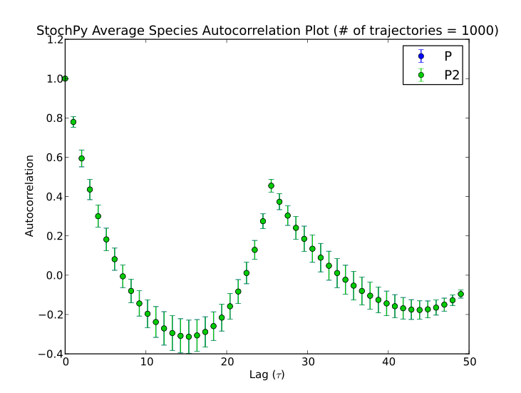
StochPy can also calculate average autocorrelations. An example is shown for the models dsmts-003-03 and dsmts-003-04:
>>> smod.Model('dsmts-003-03.xml.psc')
>>> smod.DoStochSim(end=50,mode='time',trajectories=1000)
>>> smod.GetRegularGrid()
>>> smod.PlotAverageSpeciesTimeSeries()
>>> smod.GetSpeciesAutocorrelations()
>>> smod.PlotAverageSpeciesAutocorrelations()
>>> smod.Model('dsmts-003-04.xml.psc')
>>> smod.DoStochSim(end=50,mode='time',trajectories=1000)
>>> smod.GetRegularGrid()
>>> smod.PlotAverageSpeciesTimeSeries()
>>> smod.GetSpeciesAutocorrelations()
>>> smod.PlotAverageSpeciesAutocorrelations()
Cell division is a stochastic process which can have a significant impact on molecular copy numbers in single-cells. For this reason, we developed a cell division module for StochPy where we incorporate cell division events into a stochastic simulation. In reality, the numbers of cells increases with 2^n whereas, within StochPy, we simulate the time evolution of one particular cell. In other words, we track one cell lineage over time. Interestingly, under certain conditions we can use the cell lineage to get information about the cell population. More on this later.

We can start our cell division module with the following command:
>>> cmod = stochpy.CellDivision()
By default, StochPy starts loading the model ‘CellDivision.psc’ which describes protein synthesis inside the cell. The StochPy cell division module continues simulating one cell lineage until the number of specified generations, time steps or end time is reached. Modeling of cell division is an example of sequential simulations where each generation starts with the output of the previous generation. This makes these sequential simulations more tricky than doing parallel simulations which is generally easy for most stochastic simulator software packages.
Doing a stochastic simulation with explicit cell division requires setting growth and division properties. An overview of these settings is shown in the table below. Without specifying these settings, StochPy will exploit the default settings shown in the last column.
| Description | StochPy Function | Mandatory Arguments (defaults) |
|---|---|---|
| Growth Function | SetGrowthFunction(growth_rate,growth_type) | (1.0, ‘exponential’) |
| Initial Cell Volume | SetInitialVolume(initial_volume) | 1.0 |
| Exact Dividing Species | SetExactDividingSpecies(species) | [] |
| Non Dividing Species | SetNonDividingSpecies(species) | [] |
| Set Volume Dependencies | SetVolumeDependencies(IsVolumeDependent, VolumeDependencies,SpeciesExtracellular) | True, [],[] |
| Division properties | SetVolumeDistributions(phi,K) | (‘beta’,5,5), (‘beta’,2,2),2) |
Most functionalities are relatively straightforward to use, but we discuss each of them here extensively.
This means that, for instance, phi = (‘fixed’, 2) and K = (‘fixed’,0.5) creates a cell lineage where each cells grows from a volume of 1 to 2 (assuming that we also have a initial cell volume of 1). For both distributions, we use by default a beta distribution which is defined on the interval [0,1]. This beta-distribution is symmetrical around 0.5 if both shape parameters are identical.
We will now illustrate how we use these beta distributions:
>>> SetVolumeDistributions(phi = ('beta',5,5), K = ('beta',2,2), phi_beta_mean = 2)
In this example, we set a broad distribution for both phi and K, and specified a mean of 2. The latter means that the cell division event is triggered on average at a mother cell volume of 2. We first calculate the phi_shift: phi_shift = phi_beta_mean - 0.5 = 2 -0.5 = 1.5. Next, we can determine the distributions for the mother volume at cell division
![phi = beta(5,5) + phi_{shift} = [0,1] + 1.5 = [1.5,2.5]](_images/math/6913d5e7445607aad0b04a58b90c17d94dd6b85b.png)
and the partitioning distribution
![K = \frac{beta(2,2) \times (phi_{shift} - 1) + 1}{phi_{shift} + 1} = \frac{[0,1] \times 0.5 + 1 }{2.5} = [0.4,0.6]](_images/math/1dd80ef6de95648c84b1e352ebf43bf5d2145f8e.png)
From this, we can calculate the daughter volume just after the cell division event.
![V_{daughter,1} = V_{mother} \times K = [1.5,2.5] \times [0.4,0.6] = [0.6,1.5]](_images/math/6e8bc658bb13d8d50d2e52dbba6a7a749d8c4f30.png)
In summary, the mother cell volume at division will be between [1.5,2.5] and the daughter cell volume after division will be between [0.6,1.5] for these settings.
After specifying the (default) settings, we can start a stochastic simulation with explicit cell division in. An overview of this approach is shown in the following figure.

This simulation starts with drawing a mother end volume from the specified mother volume distribution. Next, StochPy calculates the interdivision time which follows from the chosen growth rate and type of growth function. Subsequently, the stochastic simulation continues until (i) the number of time steps or the end time specified is reached or (ii) the mother cell end volume is reached. In the first case, the simulation stops. Alternatively, cell division takes place which starts with dividing the mother cell volume into two daughters. This division depends on the user specified phi (the mother cell volume distribution). In addition, each species is binomially distributed (weighted by daughter cell volume) between both daughter cells. Then, a next mother end volume is drawn and one of the daughters is selected for the next generation. Here, the largest daughter cell is more likely to be selected, because this cell will reach the next mother volume faster and is therefore likely to have more descendants. This process continues until StochPy reaches the specified number of generations, time steps or end time. An overview of method is shown above.
Example 1
We will demonstrate the incorporation of cell division for different example models. The first example considers the model ‘CellDivision.psc’ with all default specifications (growth rate, initial cell volume etc.).:
>>> cmod.DoCellDivisionStochSim()
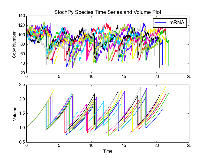
This model consists of four species, TF, TFactive, mRNA, and Protein. In addition to the existing high-level functions of the stochastic simulation module, several new functionalities are provided within the cell division module. An example is plotting of both species and volume time series:
>>> cmod.PlotSpeciesVolumeTimeSeries()

This time series plot illustrates the effect of cell division. At division, the number of proteins in the cell is binomially distributed between two daughter cells. Note that we now show species amounts, but we can use the argument plottype=’concentrations’ to get species concentrations:
>>> cmod.PlotSpeciesVolumeTimeSeries('concentrations')
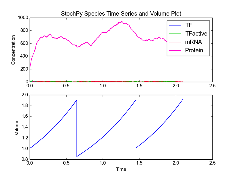
In the volume time series plot, we show the cell volume you expect based on a fixed growth rate. Importantly, in the stochastic simulation cell volume is only updated if a reaction fires. This means that we underestimate the time until a volume-dependent reaction fires. The reason is that we calculate the volume-dependent propensities with a volume smaller than the volume at the time of the reaction. If we correct for additional volume growth, we would get on average an increased time until firing for these volume-dependent reactions. However, this error is typically very small, because most models have at least one reaction that fires frequently. The error can even be zero if there are no second or higher-order reactions (zero and first order reactions are not volume dependent).
We can do any type of analysis that is also possible in the SSA module. An example is calculating the mean and standard deviation of each species. Note that this is the species mean of the lineage, not the species mean of the extant population (which we can also calculate but more on this later):
>>> cmod.PrintSpeciesMeans()
Species       Mean
TF            1.045
TFactive      9.494
mRNA          8.654
Protein       1075.784
>>> cmod.PrintSpeciesStandardDeviations()
Species       Standard Deviation
TF            1.036
TFactive      2.644
mRNA          2.783
Protein       314.229
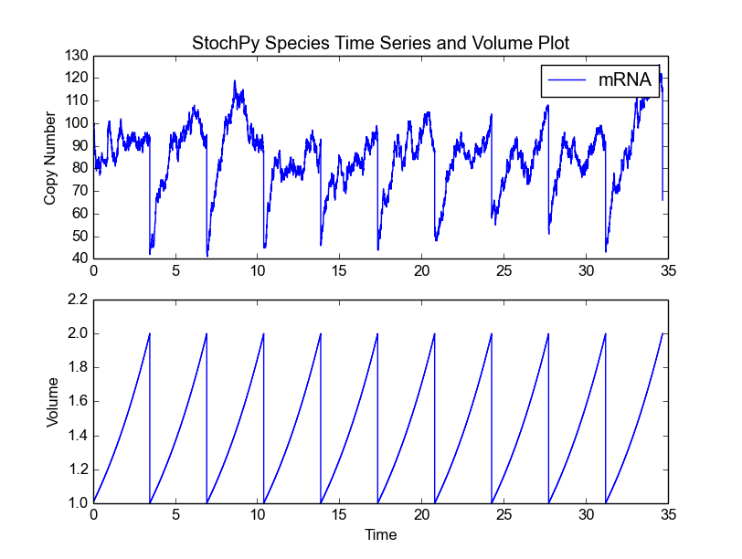
Example 2
Now, we use the ‘ImmigrationDeath.psc’ model to illustrate some more functionalities of the cell division module. After selecting the model, we modify the initial species amount and both parameters:
>>> cmod.Model('ImmigrationDeath.psc')
>>> cmod.ChangeInitialSpeciesAmount('mRNA',100)
>>> cmod.ChangeParameter('Ksyn',100)
>>> cmod.ChangeParameter('Kdeg',1)
Next, we select an exponential growth rate of 0.2 and start a simulation of 10 generations. We subsequently plot the species amounts and cell volume:
>>> cmod.SetVolumeDistributions(phi = ['fixed',2], K = ['fixed',.5])
>>> cmod.SetGrowthFunction(0.2)
>>> cmod.DoCellDivisionStochSim(end=10, mode='generations')
>>> cmod.PlotSpeciesVolumeTimeSeries('amounts')
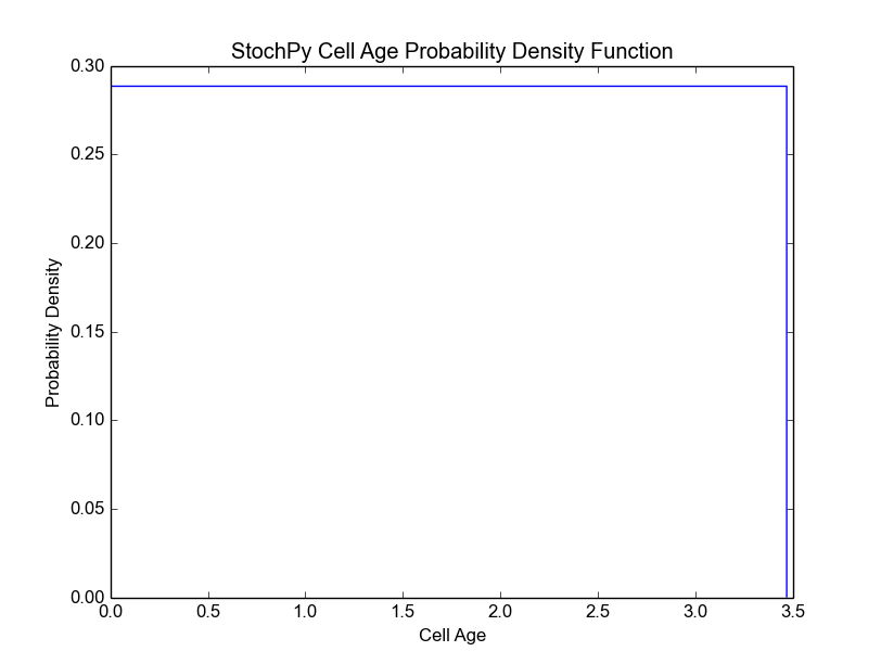
The cell division module offers the analysis of many cell division features: e.g. mother and daughter cell volume distributions, cell age distributions, interdivision time distributions, extant species distributions. For each of these statistics, we need to do a simulation for many generations to get an accurate description. Therefore, we now do a simulation for 2000 generations (which should take about a minute to simulate).
>>> cmod.DoCellDivisionStochSim(end=2000, mode='generations')
In this example, we fixed both the mother volume at cell division (2) and the partitioning of cell volume (0.5). As a result, the mother volume is always 2 and the daughter volume after division is always 1. Since we have a fixed growth rate, we also get a fixed interdivision time for each generation. This results in the following cell age distribution, i.e. all cells divide at the same age:
>>> cmod.PlotCellAgeDistribution()
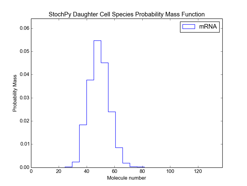
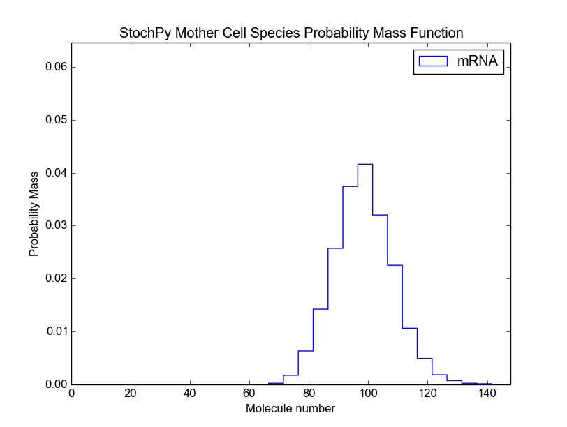
For both the mother and daughter cell, we can, for each species, determine the copy number at the moment of division (we assume that the division occurs instantly). This is shown in the next two plots for the mother and the selected daughter, respectively. The default bin size is 1, but we use a bin size of 5 here to get a better looking distribution.
>>> cmod.PlotSpeciesDaughterDistributions(bin_size=5)
>>> cmod.PlotSpeciesMotherDistributions(bin_size=5)
If certain conditions are met, we can analyze the species statistics for a population of extant cells. More specifically, we have to meet two conditions. The first condition requires that both the mother and daughter cell volume distributions are independent. Dependency occurs when a daughter is larger than the mother volume, and thus not all volumes from the mother volume distribution can be chosen. Independence can be achieved by choosing the mother cell distribution (phi) and partition distribution (K) such that there is no overlap possible between mother and daughter cell volumes. The simplest way to do this is by choosing a beta distribution for both phi and K, because this distribution is bounded between 0 and 1 (in contrast to a normal distribution, which is has no bounds). The second condition is that the single lineage is representative for the whole population. Therefore, the decision which of the two daughters to follow after division has to be made according to how many descendants each daughter cell would contribute to a later extant population.
Satisfying the first condition depends on the phi and K provided by the user, but StochPy makes sure to select the right daughter cell after division. If both conditions are met, we can use the following high-level function to get the statistics of the extant cell population:
>>> cmod.AnalyzeExtantCells(integration_method='Riemann')
We use binning and numerical integration to create the extant cell population. For numerical integration, we use two methods: (i) 2D trapezoidal rule and (ii) the Riemann sum. Both choosing the right number of bins and the right numerical integration method is important for getting accurate results. Here, we used the default number of bins and the Riemann sum method (which is typically less accurate, but not for this example). We will discuss the differences in more detail in the next example. Please use SumExtantSpeciesDistributions() to test the accuracy of the extant cell population:
>>> cmod.SumExtantSpeciesDistributions()
mRNA 1.000
For each species in your model, the printed value (sum of the extant species distribution) should be close to 1. If not, modify the number of bins. In the next example, we will demonstrate this in more detail. Since the value is very close to 1, we can continue and plot the extant cell population distribution:
>>> cmod.PlotSpeciesExtantDistributions(bin_size=5)
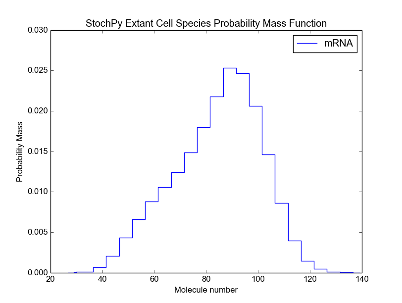
We can also calculate the mean and standard deviation of each species in the extant population:
>>> cmod.PrintSpeciesExtantMeans()
Species       Standard Deviation
mRNA          83.064

>>> cmod.PrintSpeciesExtantStandardDeviations()
Species       Standard Deviation
mRNA          16.731
These values match the expected mean and standard deviation of 83.33 and 16.57, respectively. Note that we calculated here the mean and standard deviation of the extant cell population. We can, of course, also determine these for the cell lineage:
>>> cmod.PrintSpeciesMeans()
Species       Mean
mRNA          85.708
>>> cmod.PrintSpeciesStandardDeviations()
Species       Standard Deviation
mRNA          15.985
In this particular case, they are slightly different, i.e. the mean of the cell lineage is slightly higher and the standard deviation is slightly lower.
Example 3
In this third example, we will use a beta distribution of both mother volume at division and the partitioning of this volume between both daughters. All other settings are identical to that of the previous example:
>>> cmod.Model('ImmigrationDeath.psc')
>>> cmod.ChangeInitialSpeciesAmount('mRNA',100)
>>> cmod.ChangeParameter('Ksyn',100)
>>> cmod.ChangeParameter('Kdeg',1)
Next, we select an exponential growth rate of 0.2 and start a 10 trajectory simulation of 6 generations each. We subsequently plot the species amounts and cell volume:
>>> cmod.SetGrowthFunction(0.2, 'exponential')
>>> cmod.SetInitialVolume(1)
>>> cmod.SetVolumeDistributions(phi = ['beta',2,2], K = ['beta',5,5],
    phi_beta_mean = 2)
>>> cmod.DoCellDivisionStochSim(end=6, mode='generations', trajectories = 10)
>>> cmod.PlotSpeciesVolumeTimeSeries('amounts')
Here, we simulate one trajectory (one lineage) for 10000 generations such that we can analyze some of the features of this module in more detail:
>>> cmod.ChangeParameter('Ksyn',100)
>>> cmod.ChangeParameter('Kdeg',1)
>>> cmod.SetGrowthFunction(0.2, 'exponential')
>>> cmod.SetVolumeDistributions(phi = ['beta',2,2], K = ['beta',5,5],
    phi_beta_mean = 2)
>>> cmod.DoCellDivisionStochSim(end=10000, mode='generations')
This simulation involves taking about 6.5 million time steps (including 10.000 division events) and will therefore take a few minutes to finish. In contrast to the previous example, we used a non-fixed volume of division and partitioning of mother cell volume. We set the volume distributions such that the mother volume will be beta distributed between 1.5 and 2.5 with a mean around 2.0. The daughter volume is therefore distributed between 0.6 and 1.5 (see above). We will further illustrate this by plotting both the mother and daughter cell volume:
>>> import numpy as np
>>> cmod.PlotVolumeDaughterDistributions(bins=np.linspace(0.6,1.5,10) )
>>> cmod.PlotVolumeMotherDistributions(bins=np.linspace(1.5,2.5,11) )
We decided not to use the default settings, since we now the expected range for both distributions. Note that we use here for the first time the argument bins. This argument can function as a range (as shown above) or as an integer number of bins (the default is 10). For plotting of volume, interdivision time, and cell age distributions, we use bins as argument. For all other distribution plots, we use bin_size of which plotting species number distributions is an example. The reason is that species numbers are discrete and it’s therefore convenient to think in the size of the bin rather than the number of bins. For instance, we use *bin_size*=1 as default value.
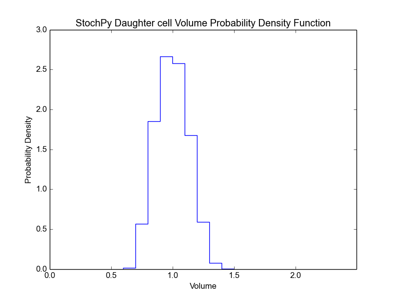
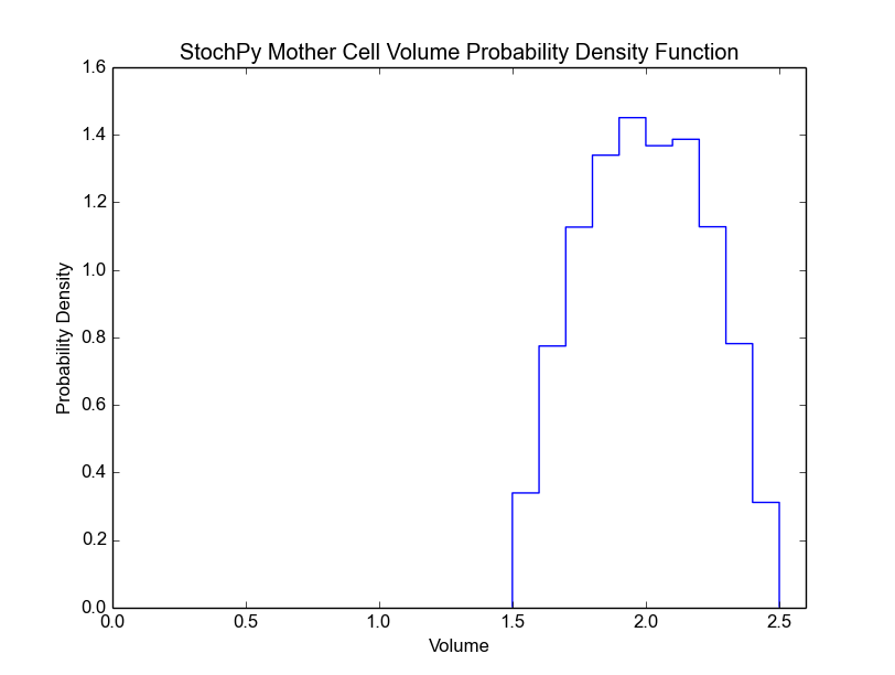
Non-fixed daughter and mother cell volumes after and at division result in different interdivision times for different generations. The distribution of these interdivision times is shown in the next plot. Additionally, we show the related cell age distribution which shows that the majority of cells divided before they reached an age of 4 time units:
>>> cmod.PlotInterdivisionTimeDistribution()
>>> cmod.PlotCellAgeDistribution(bins=100)
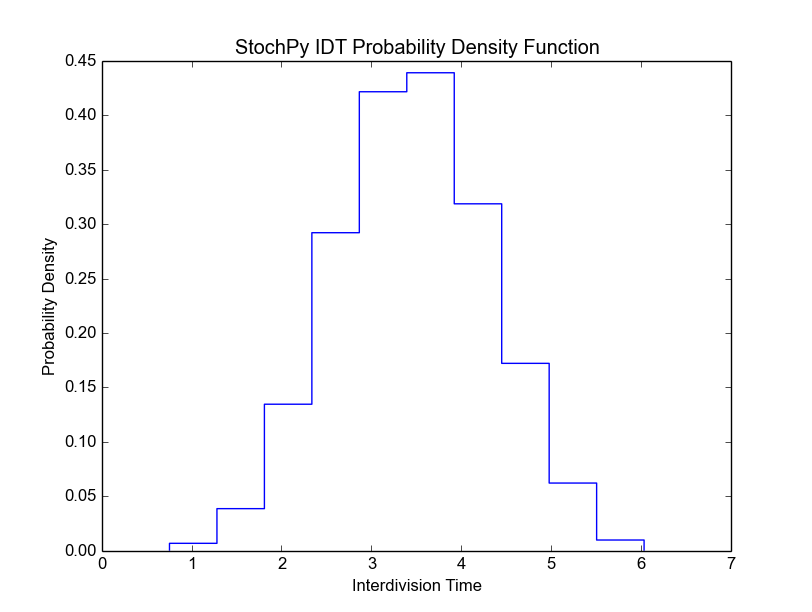
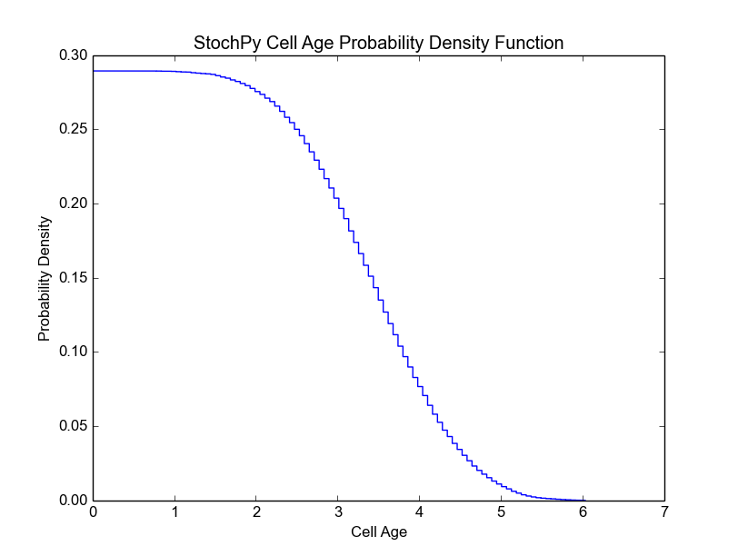
Again both conditions for analyzing the extant cell population are met, so we can analyze the copy number probabilities in the extant cell population. We determine these values via numerical integration, thus we make an approximation error. For an accurate approximation, we need to use the “right” number of bins. The right number of bins will be different for each simulation, but we use 15 as default for both cell ages and interdivision times. AnalyzeExtantCells() will return a warning message if the sum of copy number probabilities deviates too much from 1.
For numerical integration, StochPy exploits a 2D-trapezoidal rule, but we also offer the typically less accurate Riemann sum approximation method (see previous example):
>>> cmod.AnalyzeExtantCells()
Here, we did not get any warning message, because the error was within the predefined 5% error bounds. We can check the sum of species probabilities via the following function:
>>> cmod.SumExtantSpeciesDistributions()
mRNA 1.019
We made a 1.9% overestimation. Let’s use different bin settings to get more accurate species probabilities in the extant cell population. First, we show an example where the error increased:
>>> cmod.AnalyzeExtantCells(25,50)
UserWarning: We found a sum of species probabilities 0.884 in the extant cells
which is not between the desired bounds (0.95,1.05).
Our advice is to specify a different   number of bins for both age and interdivision times.
We made a relatively large error, so we got the earlier mentioned warning message. After playing a bit with the number of bins, we got a very accurate result:
>>> cmod.AnalyzeExtantCells(10,15)
>>> cmod.SumExtantSpeciesDistributions()
mRNA 0.999
Since we accurately determined the species probabilities in the extant cell population, we can now continue plotting these probabilities:
>>> cmod.PlotSpeciesExtantDistributions(bin_size=5)
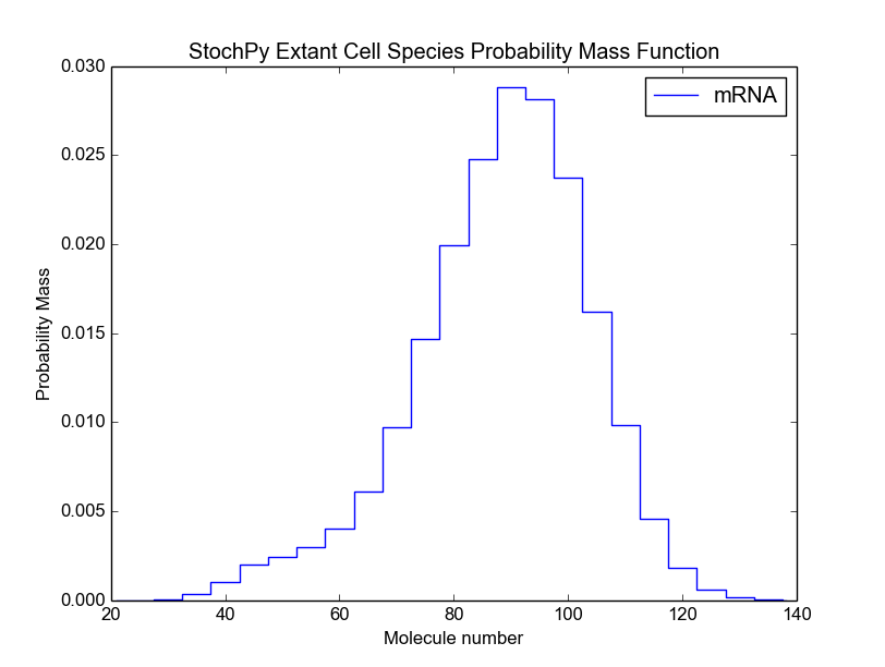
This gives the following mean and standard deviation of mRNA in the extant cell population:
>>> cmod.PrintSpeciesExtantMeans()
Species Mean
mRNA  86.777
>>> cmod.PrintSpeciesExtantStandardDeviations()
Species       Standard Deviation
mRNA  16.588
Example 4
In the last example, we use again the immigration-death model, but with completely different settings. For instance, we now use a linear growth rate and we set mRNA as ans exact dividing species. We modify some parameters and simulate the system for 25 generations. Similar to the second example, we used fixed volume distributions, which explains why division occurred at exactly a volume of 2 and why all daughter cells have a volume of exactly 1 right after division. We finally show a plot where we illustrate the concentration of mRNA as a function of time. This plot demonstrates that the concentration (not copy number) of mRNA reaches steady-state around 600.
>>> cmod.Model('ImmigrationDeath.psc')
>>> cmod.SetGrowthFunction(1./60,'linear')
>>> cmod.SetInitialVolume(1)
>>> cmod.SetVolumeDistributions(phi = ['fixed',2], K = ['fixed',.5])
>>> cmod.SetExactDividingSpecies(['mRNA'])
>>> cmod.ChangeParameter('Ksyn',10) #/min
>>> cmod.ChangeParameter('Kdeg',0)
>>> cmod.ChangeInitialSpeciesAmount('mRNA',900)
>>> cmod.DoCellDivisionStochSim(end=25, mode='generations', trajectories = 1)
>>> cmod.PlotSpeciesVolumeTimeSeries()
>>> cmod.PlotSpeciesTimeSeries('concentration',species2plot = 'mRNA',
    colors=['blue'])
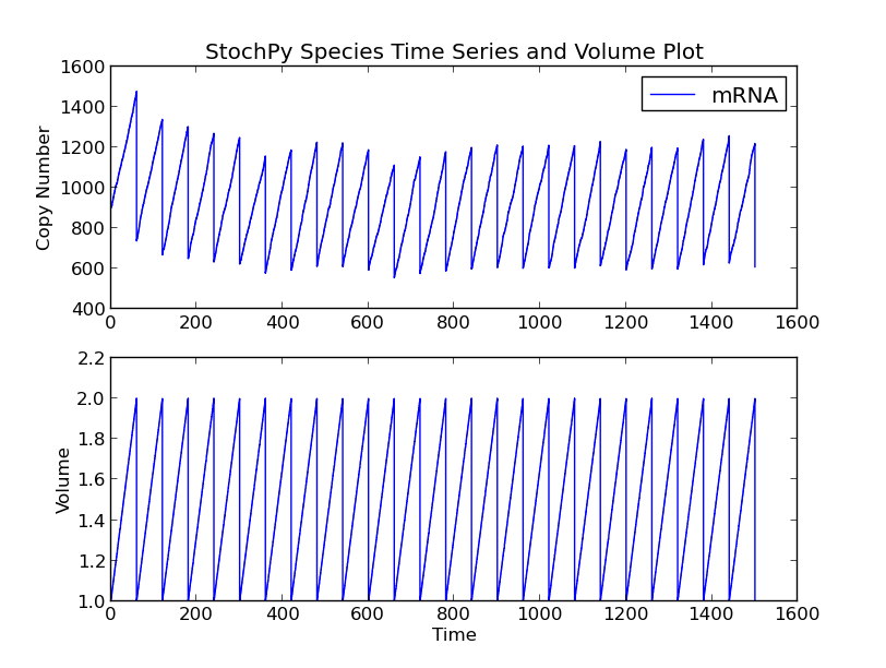
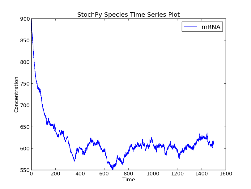
Models are often described in the SBML format, which makes it difficult to interpret. StochPy offers the SBML2PSC module that can used to convert models written in SBML to models written in the human interpretable PySCeS MDL:
>>> sbml2psc_mod = stochpy.SBML2PSC()
>>> sbml2psc_mod.SBML2PSC(sbmlfile='dsmts-003-03.xml',
sbmldir=stochpy.model_dir, pscfile=None, pscdir=None)
csymbol time defined as "t" in event
Info: single compartment model: locating "Dimerisation" in def. compartment
Info: single compartment model: locating "Disassociation" in def. compartment
Writing file: /home/user/Stochpy/pscmodels/dsmts-003-03.xml.psc

SBML2PSC
in : /home/user/Stochpy/pscmodels/dsmts-003-03.xml
out: /home/user/Stochpy/pscmodels/dsmts-003-03.xml.psc
The PySCeS MDL (see the PySCeS Model Description Language section) is the default model description format, but StochPy can parse SBML models.
StochPy (since version 2.1.0) is now available for both Python 2 (2.6+) and Python 3 (3.4+). We currently recommend to use Python 2.7. In addition to Python 2 or 3, the NumPy library is required before installing StochPy.
The following software is optional but recommended:
Matplotlib is useful for the generation of plots and libSBML is necessary to convert models written in SBML format to the PySCeS MDL. The libSBML software requires a XML parser library which is libxml2 by default.
On Ubuntu you can use the following code to directly install all required packages on Python 2.6+:
sudo apt-get install python-dev python-numpy
sudo apt-get install python-scipy python-matplotlib  python-pip
sudo apt-get install ipython ipython-notebook
sudo apt-get install libxml2 libxml2-dev
sudo apt-get install zlib1g zlib1g-dev
sudo apt-get install bzip2 libbz2-dev
sudo pip install python-libsbml
and for Python 3.4+:
sudo apt-get install python3-dev python3-numpy
sudo apt-get install python3-scipy python3-matplotlib  python3-pip
sudo apt-get install ipython3 ipython3-notebook
sudo apt-get install libxml2 libxml2-dev
sudo apt-get install zlib1g zlib1g-dev
sudo apt-get install bzip2 libbz2-dev
sudo pip3 install python-libsbml
Download the windows installer (32-bit) or the source code and use setup.py.
Python 2.6.x:
python setup.py install
Python 3.4.x:
python3 setup.py install
Note that you can also generate your own windows installer:
python setup.py bdist_wininst
Download the source code and use setup.py
In the command line,:
cd /.../StochPy-2.2.0
Python 2:
sudo python setup.py install
Python 3:
$ sudo python3 setup.py install
The StochPy package contains some example models, such as:
The files describing these models can be found in the directory /home dir/Stochpy/pscmodels/ after the first usage of the package. Most of these models are written in the PySCeS MDL format. This PySCeS MDL is explained in the PySCeS Model Description Language section. Besides PySCeS MDL, StochPy also accepts models written in SBML.
In this section, we compare deterministic and stochastic rate equations. In short, zero and first order rate equations will be identical, but second and higher order reactions are different if a two or more of the same species are necessary for the reaction to take place (e.g. 2X > Y).
Deterministic models represent species often by concentration, while stochastic models represent species often by amounts. The species amounts are identical to:
Na*[X]*Volume(L)
Here, Na is the number of Avegadro (6.02*10e23). This is the first step of the conversion of deterministic rate constants (k) to stochastic rate constants (c).
Assume the following reaction:
--> X
The deterministic rate equation of this reaction is:
k (Ms^-1)
The stochastic rate equation of this reaction is:
c (s^-1)
Consider the following reaction:
X --> Y
The deterministic rate equation of this reaction is:
k*[X]
The stochastic rate equation of this reaction is:
c*x (s^-1)
Here, x corresponds to Na*[X]*Volume(L) particles. Therefore, x changes k*Na*[X]*Volume(L) = k*x molecules per second, which means that k=c. This means that first order stochastic and deterministic rate equations are identical.
There exist several types of second-order reactions. First, consider the next reaction:
X+Y --> Z
The deterministic rate equation of this reaction is:
k*[X]*[Y] (Ms^-1)
The stochastic rate equation of this reaction is:
c*x*y (s^-1)
Again, [X] corresponds to Na*[X]*Volume(L) particles and the same is true for [Y]. Therefore, the following relationship holds:
k*[X]*[Y] (Ms^-1) = (k*x*y)/(Na*V)^2, hence c = k/(Na*V)
Secondly, consider a dimerization reaction:
2X --> Y
The deterministic rate equation of this reaction is:
k*X^2
The stochastic rate equation of this reaction is:
0.5*c*x*(x-1)
The first important concept to understand is that a dimerization reaction can only occur if there are at least two molecules of species X available. For this reason, the stochastic rate equation must be zero if there is only one X molecule available.
This type of reactions does usually not occur in chemical reactions, but they are described just for the sake of completeness.
There exist three types of third-order reactions
1) X+Y+Z –> A
The deterministic rate equation of this reaction is:
k*[X]*[Y]*[Z]
The stochastic rate equation of this reaction is:
c*x*y*z
2) X+2Y –> Z
The deterministic rate equation of this reaction is:
k*[X]*([Y]^2)
The stochastic rate equation of this reaction is:
0.5*c*x*y*(y-1)
3) 3X –> Y
The deterministic rate equation of this reaction is:
k*[X]^3
The stochastic rate equation of this reaction is:
(1/6)*x*(x-1)*(x-2)
For the last reaction three x molecules are necessary, thus this rate equation can not fire if there are less than three molecules of x available.