datamanager - easy access to and manipulation of data¶

The datamanager classes and functions are useful for locating the correct data file for a particular day and manipulating data and subsets in a generic way.

Authors: Jon Niehof

Institution: University of New Hampshire

Contact: Jonathan.Niehof@unh.edu

About datamanager¶

Examples¶

Examples go here

Classes

DataManager(directories, file_fmt[, ...])

THIS CLASS IS NOT YET COMPLETE, doesn't do much useful.

Functions

`apply_index`(data, idx)	Apply an array of indices to data.
`array_interleave`(array1, array2, idx)	Create an array containing all elements of both array1 and array2
`axis_index`(shape[, axis])	Returns array of indices along axis, for all other axes
`flatten_idx`(idx[, axis])	Convert multidimensional index into index on flattened array.
`insert_fill`(times, data[, fillval, tol, ...])	Populate gaps in data with fill.
`rebin`(data, bindata, bins[, axis, bintype, ...])	Rebin one axis of input data based on values of another array
`rev_index`(idx[, axis])	From an index, return an index that reverses the action of that index
`values_to_steps`(array[, axis])	Transform values along an axis to their order in a unique sequence.

class spacepy.datamanager.DataManager(directories, file_fmt, descend=False, period=None)[source]¶

THIS CLASS IS NOT YET COMPLETE, doesn’t do much useful.

Will have to do something that allows the config file to specify regex and other things, and then just the directory to be changed (since regex, etc.

Parameters:

directorieslist: A list of directories that might contain the data
file_fmtstring: Regular expression that matches the files desired. Will also recognize strftime parameters %w %d %m %y %Y %H %M %s %j %U %W, all zero-pad. https://docs.python.org/2/library/datetime.html#strftime-strptime-behavior Can have subdirectory reference, but separator should be unix-style, with no leading slash.
periodstring: Size of file; can be a number followed by one of d, m, y, H, M, s. Anything else is assumed to be “irregular” and files treated as if there are neither gaps nor overlaps in the sequence. If not specified, will be assumed to match one count of the smallest unit in the format string.

files_matching(dt=None)[source]¶

Return all the files matching this file format

Parameters:

dtdatetime: Optional; if specified, match only files for this date.

Returns:

outgenerator: Iterates over every file matching the format specified at creation. Note this is specified in native path format!

get_filename(dt)[source]¶: Returns the filename corresponding to a particular point in time

spacepy.datamanager.apply_index(data, idx)[source]¶

Apply an array of indices to data.

Most useful in dealing with the output from numpy.argsort(), and best explained by the example.

Parameters:

dataarray: Input data, at least two dimensional. The 0th dimension is treated as a “time” or “record” dimension.
idxsequence: 2D index to apply to the import data. The 0th dimension must be the same size as data’s 0th dimension. Dimension 1 must be the same size as one other dimension in data (the first match found is used); this is referred to as the “index dimension.”

Returns:

datasequence: View of data, with index applied. For each index of the 0th dimension, the values along the index dimension are obtained by applying the value of idx at the same index in the 0th dimension. This is repeated across any other dimensions in data.

Warning

No guarantee is made whether the returned data is a copy of the input data. Modifying values in the input may change the values of the input. Call copy() if a copy is required.

Raises:

ValueErrorif can’t match the shape of data and indices

Examples

Assume flux is a 3D array of fluxes, with a value for each of time, pitch angle, and energy. Assume energy is not necessarily constant in time, nor is ordered in the energy dimension. If energy is a 2D array of the energies as a function of energy step for each time, then the following will sort the flux at each time and pitch angle in energy order.

>>> idx = numpy.argsort(energy, axis=1)
>>> flux_sorted = spacepy.datamanager.apply_index(flux, idx)

spacepy.datamanager.array_interleave(array1, array2, idx)[source]¶

Create an array containing all elements of both array1 and array2

idx is an index on the output array which indicates which elements will be populated from array1, i.e., out[idx] == array1 (in order.) The other elements of out will be filled, in order, from array2.

Parameters:

array1array: Input data.
array2array: Input data. Must have same number of dimensions as array1, and all dimensions except the zeroth must also have the same length.
idxarray: A 1D array of indices on the zeroth dimension of the output array. Must have the same length as the zeroth dimension of array1.

Returns:

outarray: All elements from array1 and array2, interleaved according to idx.

Examples

>>> import numpy
>>> import spacepy.datamanager
>>> a = numpy.array([10, 20, 30])
>>> b = numpy.array([1, 2])
>>> idx = numpy.array([1, 2, 4])
>>> spacepy.datamanager.array_interleave(a, b, idx)
array([ 1, 10, 20,  2, 30])

spacepy.datamanager.axis_index(shape, axis=- 1)[source]¶

Returns array of indices along axis, for all other axes

Parameters:

shapetuple: Shape of the output array

Returns:

idxarray: An array of indices. The value of each element is that element’s index along axis.

Other Parameters:

axisint: Axis along which to return indices, defaults to the last axis.

See also

apply_index

Examples

>>> import numpy
>>> import spacepy.datamanager
>>> data = numpy.array([[3, 1, 2], [3, 2, 1]])
>>> idx = numpy.argsort(data, -1)
>>> idx_flat = spacepy.datamanager.flatten_idx(idx)
>>> data.ravel() #flat array
array([3, 1, 2, 3, 2, 1])
>>> idx_flat #indices into the flat array
array([1, 2, 0, 5, 4, 3])
>>> data.ravel()[idx_flat] #index applied to the flat array
array([1, 2, 3, 1, 2, 3])

spacepy.datamanager.insert_fill(times, data, fillval=nan, tol=1.5, absolute=None, doTimes=True)[source]¶

Populate gaps in data with fill.

Continuous data are often treated differently from discontinuous data, e.g., matplotlib will draw lines connecting data points but break the line at fill. Often data will be irregularly sampled but also contain large gaps that are not explicitly marked as fill. This function adds a single record of explicit fill to each gap, defined as places where the spacing between input times is a certain multiple of the median spacing.

Parameters:

timessequence: Values representing when the data were taken. Must be one-dimensional, i.e., each value must be scalar. Not modified
datasequence: Input data.

Returns:

times, datatuple of sequence: Copies of input times and data, fill added in gaps (doTimes True)
datasequence: Copy of input data, with fill added in gaps (doTimes False)

Other Parameters:

fillval: Fill value, same type as data. Default is numpy.nan. If scalar, will be repeated to match the shape of data (minus the time axis).

Note

The default value of nan will not produce good results with integer input.
tolfloat: Tolerance. A single fill value is inserted between adjacent values where the spacing in times is strictly greater than tol times the median of the spacing across all times. The inserted time for fill is halfway between the time on each side. (Default 1.5)
absolute: An absolute value for maximum spacing, of a type that would result from a difference in times. If specified, tol is ignored and any gap strictly larger than absolute will have fill inserted.
doTimesboolean: If True (default), will return a tuple of the times (with new values inserted for the fill records) and the data with new fill values. If False, will only return the data – useful for applying fill to multiple arrays of data on the same timebase.

Raises:

ValueErrorif can’t identify the time axis of data: Try using numpy.rollaxis() to put the time axis first in both data and times.

Examples

This example shows simple hourly data with a gap, populated with fill. Note that only a single fill value is inserted, to break the sequence of valid data rather than trying to match the existing cadence.

>>> import datetime
>>> import numpy
>>> import spacepy.datamanager
>>> t = [datetime.datetime(2012, 1, 1, 0),
         datetime.datetime(2012, 1, 1, 1),
         datetime.datetime(2012, 1, 1, 2),
         datetime.datetime(2012, 1, 1, 5),
         datetime.datetime(2012, 1, 1, 6)]
>>> temp = [30.0, 28, 27, 32, 35]
>>> filled_t, filled_temp = spacepy.datamanager.insert_fill(t, temp)
>>> filled_t
array([datetime.datetime(2012, 1, 1, 0, 0),
       datetime.datetime(2012, 1, 1, 1, 0),
       datetime.datetime(2012, 1, 1, 2, 0),
       datetime.datetime(2012, 1, 1, 3, 30),
       datetime.datetime(2012, 1, 1, 5, 0),
       datetime.datetime(2012, 1, 1, 6, 0)], dtype=object)
>>> filled_temp
array([ 30.,  28.,  27.,  nan,  32.,  35.])

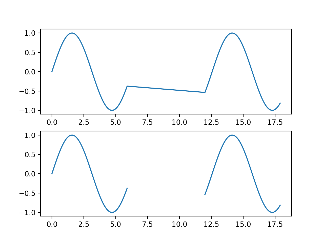
This example plots “gappy” data with and without explicit fill values.

>>> import matplotlib.pyplot as plt
>>> import numpy
>>> import spacepy.datamanager
>>> x = numpy.append(numpy.arange(0, 6, 0.1), numpy.arange(12, 18, 0.1))
>>> y = numpy.sin(x)
>>> xf, yf = spacepy.datamanager.insert_fill(x, y)
>>> fig = plt.figure()
>>> ax0 = fig.add_subplot(211)
>>> ax0.plot(x, y)
>>> ax1 = fig.add_subplot(212)
>>> ax1.plot(xf, yf)
>>> plt.show()

(Source code, png, hires.png, pdf)

spacepy.datamanager.rebin(data, bindata, bins, axis=- 1, bintype='mean', weights=None, clip=False, bindatadelta=None)[source]¶

Rebin one axis of input data based on values of another array

This is clearest with an example. Consider a flux as a function of time, energy, and the look direction of a detector (could be multiple detectors, or spin sectors.) The flux is then 3-D, dimensioned Nt x Ne x Nl. Now consider that each look direction has an associated pitch angle that is a function of time and thus stored in an array Nt x Nl. Then this function will redimension the flux into pitch angle bins (rather than tags.)

So consider the PA bins to have dimension Np + 1 (because it represents the edges, the number of bins is one less than the dimension.) Then the output will be dimensioned Nt x Ne x Np.

bindata must be same or lesser dimensionality than data. Any axes which are present must be either of size 1, or the same size as data. So for data 100x5x20, bindata may be 100x5x20, or 100, or 100x1x20, but not 100x20x5. This function will insert axes of size 1 as needed to match dimensionality.

Parameters:

datandarray: N-dimensional array of data to be rebinned. nan are ignored.
bindatandarray: M-dimensional (M<=N) array of values to be compared to the bins.
binsndarray: 1-D array of bin edges. Output dimension will be this size minus 1. Any values in bindata that don’t fall in the bins will be omitted from the output. (See clip to change this behavior).

Returns:

ndarray: data with one axis redimensioned, from its original dimension to the bin dimension.

Other Parameters:

axisint

Axis of data to rebin. This axis will disappear in the output and be replaced with an axis of the size of bins less one. (Default -1, last axis)

bintypestr

Type of rebinning to perform:

mean: Return the mean of all values in the bin (default)
unc: Return the quadrature mean of all values in the bin, for propagating uncertainty
count: Return the count of values that fall in each bin.

weightsndarray

Relative weight of each sample in bindata. Must be same shape as bindata. Purely relative, i.e. the output is only affected based on the total of weights if bintype is count. Note if weights is specified, count returns the sum of the weights, not the count of individual samples.

clipboolean

Clip data to the bins. If true, all input data will be assigned a bin and data outside the range of the bin edges will be assigned to the extreme bins. If false (default), input data outside the bin ranges will be ignored.

bindatadeltandarray

By default, the bindata are treated as point values. If bindatadelta is specified, it is treated as the half-width of the bindata, allowing a single input value to be split between output bins. Must be scalar, or same shape as bindata. Note that input values are not weighted by the bin width, but by number of input values or by weights. (Combining weights with bindatadelta is not comprehensively tested.)

Examples

Consider a particle flux distribution that’s a function of energy and pitch angle. For simplicity, assume that the energy dependence is a simple power law and the pitch angle dependence is Gaussian, with a peak whose position oscillates in time over a period of about one hour. This is fairly non-physical but illustrative.

First making the relevant imports:

>>> import matplotlib.pyplot
>>> import numpy
>>> import spacepy.datamanager
>>> import spacepy.plot

The functional form of the flux is then:

>>> def j(e, t, a):
...     return e ** -2 * (1 / (90 * numpy.sqrt(2 * numpy.pi))) \
...     * numpy.exp(
...         -0.5 * ((a - 90 + 90 * numpy.sin(t / 573.)) / 90.) ** 2)

Illustrating the flux at one energy as a function of pitch angle:

>>> times = numpy.arange(0., 7200, 5)
>>> alpha = numpy.arange(0, 181., 2)
# Add a dimension so the flux is a 2D array
>>> flux = j(1., numpy.expand_dims(times, 1),
...          numpy.expand_dims(alpha, 0))
>>> spacepy.plot.simpleSpectrogram(times, alpha, flux, cb=False,
...                                ylog=False)
>>> matplotlib.pyplot.ylabel('Pitch angle (deg)')
>>> matplotlib.pyplot.xlabel('Time (sec)')
>>> matplotlib.pyplot.title('Flux at 1 MeV')

(Source code, png, hires.png, pdf)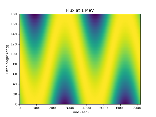

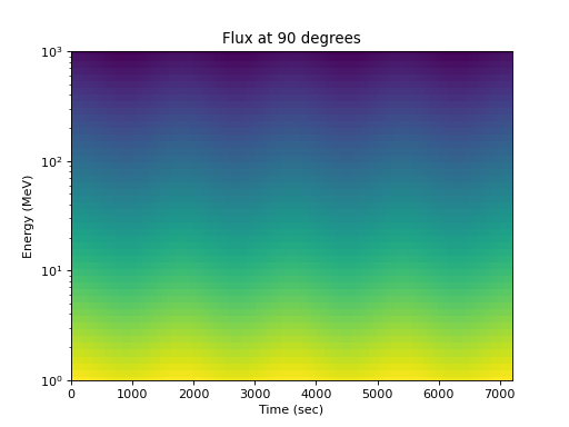
Or the flux at one pitch angle as a function of energy:

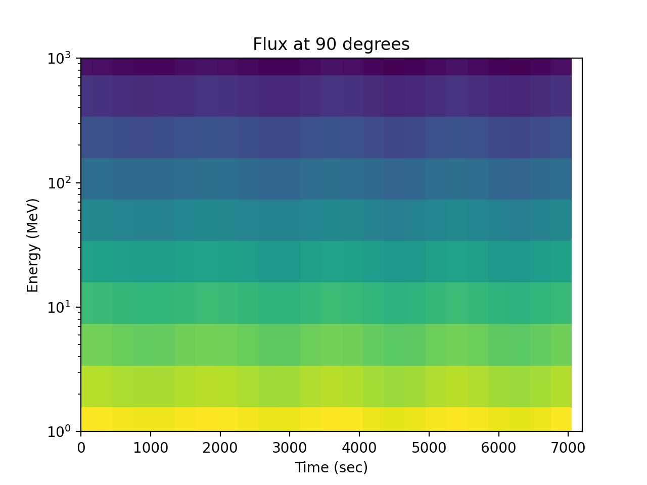
>>> energies = numpy.logspace(0, 3, 50)
>>> flux = j(numpy.expand_dims(energies, 0),
...          numpy.expand_dims(times, 1), 90.)
>>> spacepy.plot.simpleSpectrogram(times, energies, flux, cb=False)
>>> matplotlib.pyplot.ylabel('Energy (MeV)')
>>> matplotlib.pyplot.xlabel('Time (sec)')
>>> matplotlib.pyplot.title('Flux at 90 degrees')

(Source code, png, hires.png, pdf)

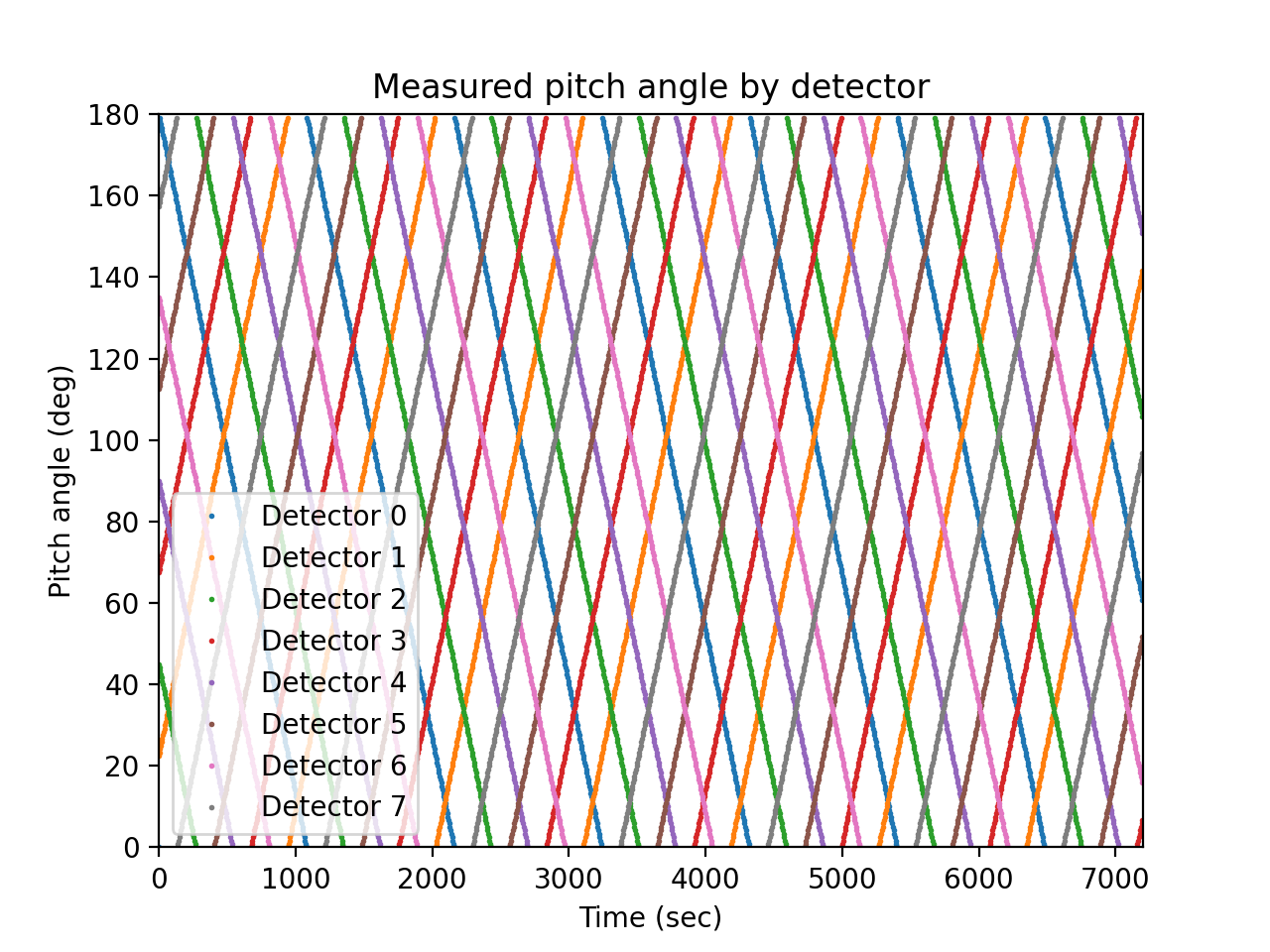
The measurement is usually not aligned with a pitch angle grid, and the detector pointing in pitch angle space usually varies with time. Taking a very simple case of eight detectors that sweep through pitch angle space in an organized fashion at ten degrees per minute, the measured pitch angle as a function of detector and time is:

>>> def pa(d, t):
...     return (d * 22.5 + t * (2 * (d % 2) - 1)) % 180
>>> lines = matplotlib.pyplot.plot(
...     times, pa(numpy.arange(8).reshape(1, -1), times.reshape(-1, 1)),
...     marker='o', ms=1, linestyle='')
>>> matplotlib.pyplot.legend(lines,
...     ['Detector {}'.format(i) for i in range(4)], loc='best')
>>> matplotlib.pyplot.xlabel('Time (sec)')
>>> matplotlib.pyplot.ylabel('Pitch angle (deg)')
>>> matplotlib.pyplot.title('Measured pitch angle by detector')

(Source code, png, hires.png, pdf)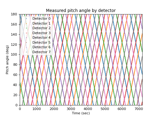

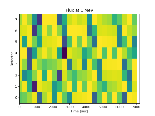
Assuming a coarser measurement in time and energy than used to illustrate the distribution above, the measured flux as a function of time, detector, and energy is constructed:

>>> times = numpy.arange(0., 7200, 300) #5 min cadence
>>> alpha = pa(numpy.arange(8).reshape(1, -1), times.reshape(-1, 1))
>>> energies = numpy.logspace(0, 3, 10) #10 energy channels (3/decade)
# Every dimension (t, detector, e) gets its own numpy axis
>>> flux = j(numpy.reshape(energies, (1, 1, -1)),
             numpy.reshape(times, (-1, 1, 1)),
             numpy.expand_dims(alpha, -1))
>>> flux.shape
(24, 8, 10)

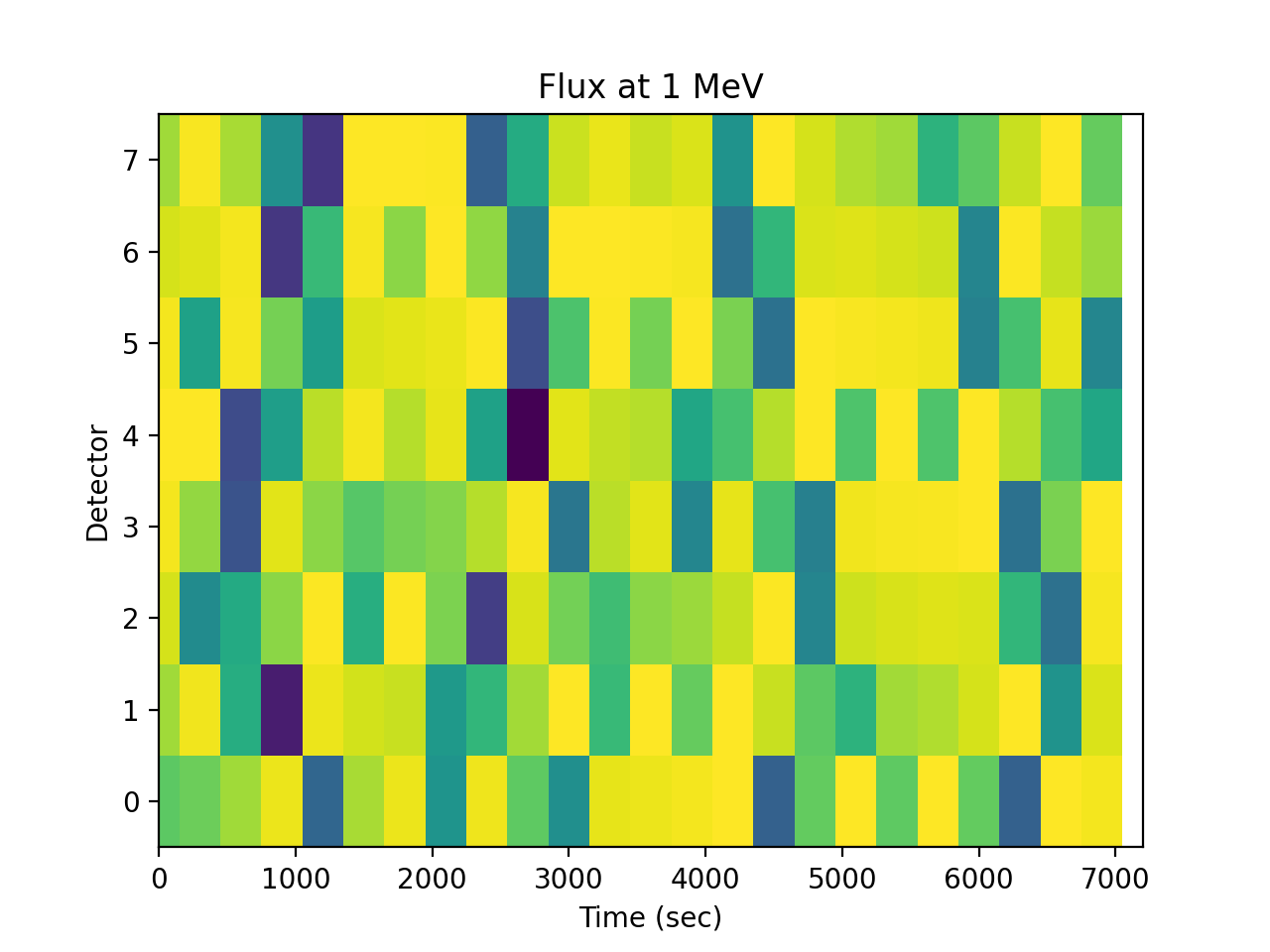
The flux at an energy as a function of detector is not very useful:

>>> spacepy.plot.simpleSpectrogram(times, numpy.arange(8),
...                                flux[..., 0], cb=False, ylog=False)
>>> matplotlib.pyplot.ylabel('Detector')
>>> matplotlib.pyplot.xlabel('Time (sec)')
>>> matplotlib.pyplot.title('Flux at 1 MeV')

(Source code, png, hires.png, pdf)

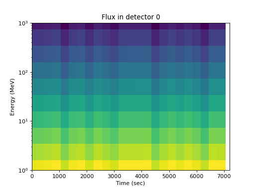
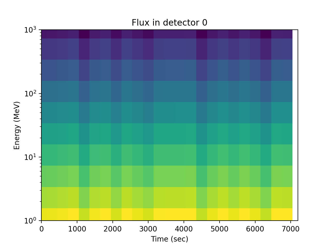
As a function of energy for one detector, the energy dependence is apparent but time and pitch angle effects are confounded:

>>> spacepy.plot.simpleSpectrogram(times, energies, flux[:, 0, :],
...                                cb=False)
>>> matplotlib.pyplot.ylabel('Energy (MeV)')
>>> matplotlib.pyplot.xlabel('Time (sec)')
>>> matplotlib.pyplot.title('Flux in detector 0')

(Source code, png, hires.png, pdf)

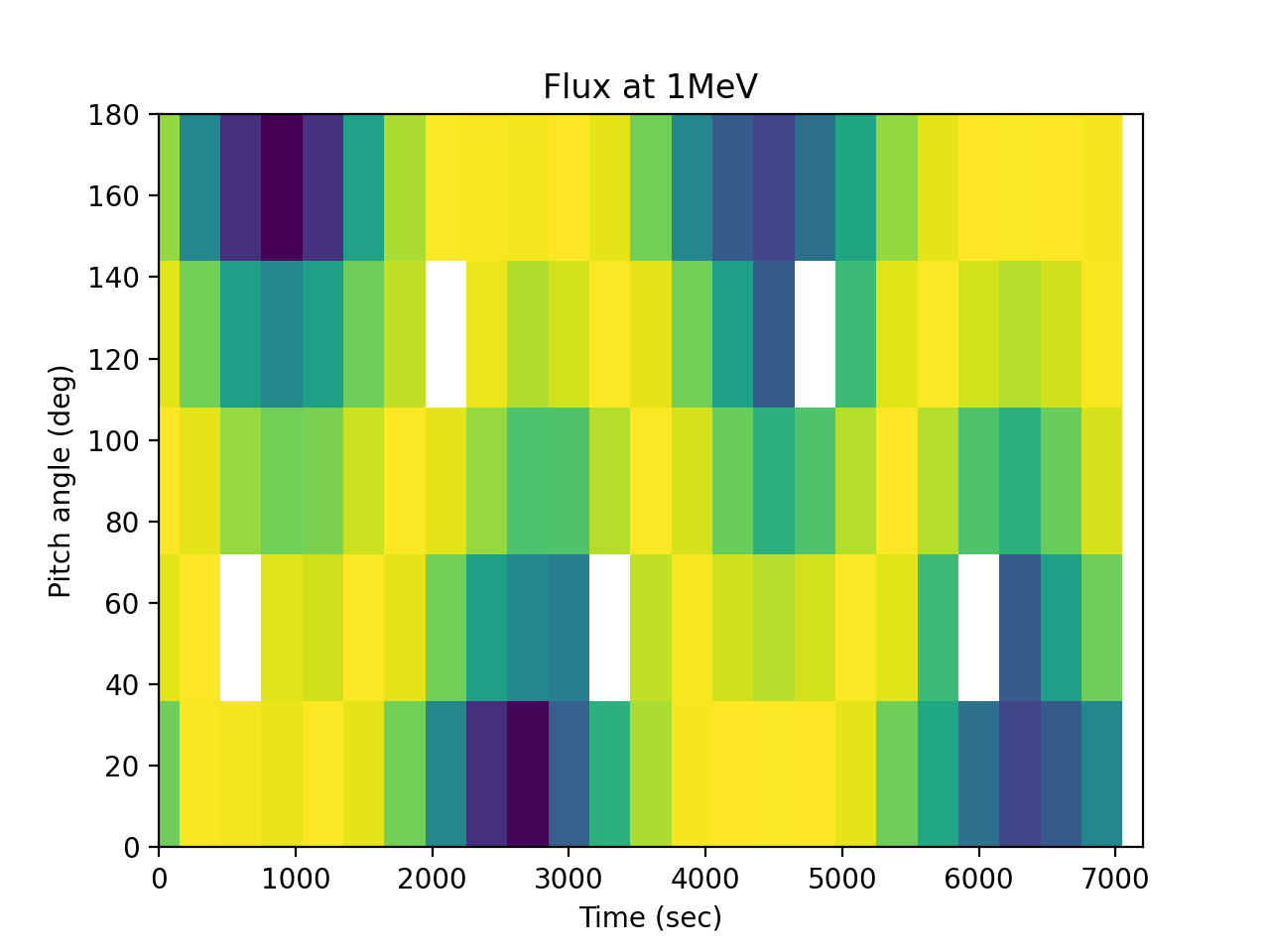
What is needed is to recover the array of flux dimensioned by time, pitch angle, and energy, with appropriate pitch angle bins. The assumption is that the pitch angle as a function of time and detector is measured and thus the alpha array is available. Using that array, rebin can change flux from time, detector, energy bins to time, pitch angle, energy bins. The axis 1 changes from a detector dimension to pitch angle:

>>> pa_bins = numpy.arange(0, 181, 36)
>>> flux_by_pa = spacepy.datamanager.rebin(
...     flux, alpha, pa_bins, axis=1)
>>> flux_by_pa.shape
(24, 6, 10)

This can then be visualized. The pitch angle coverage is not perfect, but the original shape of the distribution is apparent, and further analysis can be performed on the regular pitch angle grid:

>>> spacepy.plot.simpleSpectrogram(times, pa_bins, flux_by_pa[..., 0],
...                                cb=False, ylog=False)
>>> matplotlib.pyplot.ylabel('Pitch angle (deg)')
>>> matplotlib.pyplot.xlabel('Time (sec)')
>>> matplotlib.pyplot.title('Flux at 1MeV')

(Source code, png, hires.png, pdf)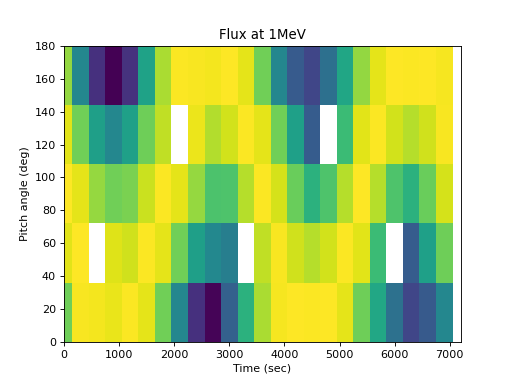

Or by energy:

>>> spacepy.plot.simpleSpectrogram(times, energies, flux_by_pa[:, 2, :],
...                                cb=False)
>>> matplotlib.pyplot.ylabel('Energy (MeV)')
>>> matplotlib.pyplot.xlabel('Time (sec)')
>>> matplotlib.pyplot.title('Flux at 90 degrees')

(Source code, png, hires.png, pdf)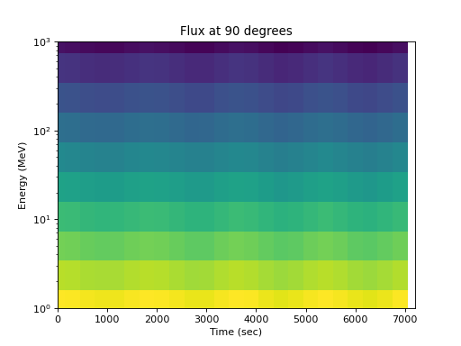

rebin can be used for higher dimension data, if the pitch angle itself depends on energy (e.g. if an energy sweep takes substantial time), and to propagate uncertainties through the rebinning. It can also be used to rebin on the time axis, e.g. for transforming time base.

spacepy.datamanager.rev_index(idx, axis=- 1)[source]¶

From an index, return an index that reverses the action of that index

Essentially, a[idx][rev_index(idx)] == a

Note

This becomes more complicated in multiple dimensions, due to the vagaries of applying a multidimensional index.

Parameters:

idxarray: Indices onto an array, often the output of argsort().

Returns:

rev_idxarray: Indices that, when applied to an array after idx, will return the original array (before the application of idx).

Other Parameters:

axisint: Axis along which to return indices, defaults to the last axis.

Table of Contents

Previous topic

Next topic

This Page

datamanager - easy access to and manipulation of data¶

About datamanager¶

Examples¶