Processing Results

DDSCAT can generate a plethora of output files. ScatPy aims to make reading and working with those files easy. The classes and functions for dealing with output files are found in the module results.

The basic class for managing output files is the Table. This has been subclassed to provide tables appropriate for the many different files that DDSCAT returns

Name	File
Table	N/A
ResultTable	N/A
QTable	qtable - Primary result table
QTable2	qtable2 - Secondary result table
MTable	mtable - Material output file
MInTable	Material input file
ShapeTable	shape.dat - Input dipole table for custom targets
TargetTable	target.out - Output dipole table
AVGTable	.avg - Scattering information for each target orientation
AVGSummaryTable	.avg - The header summary from AVGTable
SCASummaryTable	.sca - The header summary of an SCA file
EnTable	.E1 and .E2 - Nearfield results

Working with Tables

Tables in the current working directory can be opened by simply calling the appropriate class with no arguments. The table will load from the default file used by DDSCAT. For instance:

>>> q = results.QTable()
>>> q.fname
'qtable'
>>> t = results.TargetTable()
>>> t.fname
'target.out'

Tables are based on Python dicts, and columns in the file correspond to fields in the Table, with the key names corresponding to the column labels:

>>> t.keys()
['IY', 'IX', 'IZ', 'ICOMPz', 'ICOMPx', 'ICOMPy', 'JA']
>>> q.keys()
['Q_ext', 'Nsca', 'wave', 'Q_abs', '<cos^2>', 'Q_sca', 'Q_bk', 'aeff', 'g(1)=<cos>']
>>> q['wave']
array([ 0.35   ,  0.36531,  0.38061,  0.39592,  0.41122,  0.42653,
        0.44184,  0.45714,  0.47245,  0.48776,  0.50306,  0.51837,
        0.53367,  0.54898,  0.56429,  0.57959,  0.5949 ,  0.6102 ,
        0.62551,  0.64082,  0.65612,  0.67143,  0.68673,  0.70204,
        0.71735,  0.73265,  0.74796,  0.76327,  0.77857,  0.79388,
        0.80918,  0.82449,  0.8398 ,  0.8551 ,  0.87041,  0.88571,
        0.90102,  0.91633,  0.93163,  0.94694,  0.96224,  0.97755,
        0.99286,  1.0082 ,  1.0235 ,  1.0388 ,  1.0541 ,  1.0694 ,
        1.0847 ,  1.1    ])

Generally, data contained in a table will be accessed through these column fields, but it is possible to directly address the entire table through the data property:

>>> t.data
array([[    1,     1,     4, ...,     1,     1,     1],
       [    2,     1,     4, ...,     1,     1,     1],
       [    3,     1,     4, ...,     1,     1,     1],
       ...,
       [14418,    45,     9, ...,     1,     1,     1],
       [14419,    45,     9, ...,     1,     1,     1],
       [14420,    45,     9, ...,     1,     1,     1]])

Plotting Tables

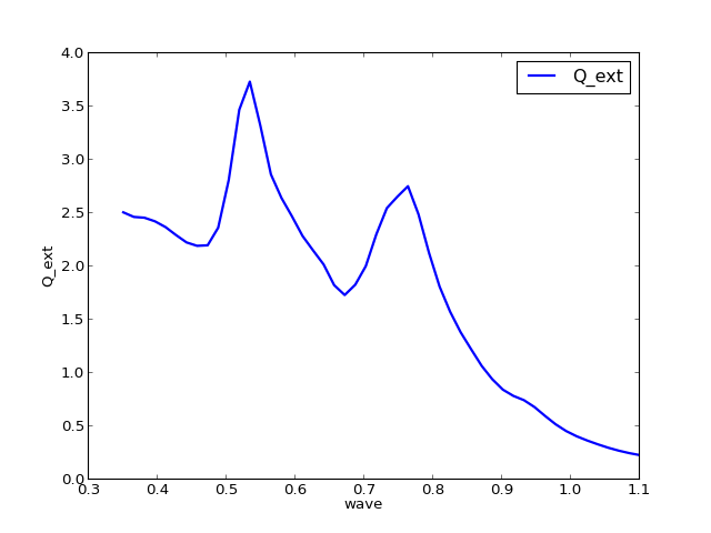
The data in a table can be visualized with the plot method.

(Source code)

q = results.QTable()
q.plot()
legend(loc=0)

(Source code, png, hires.png, pdf)

Which columns are plotted is controlled by the attributes x_field and y_fields.

>>> q.x_field
'wave'
>>> q.y_fields
['Q_ext']
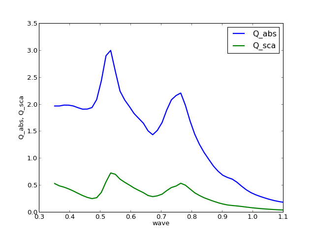
>>> q.y_fields = ['Q_abs', 'Q_sca']

clf()
q.y_fields = ['Q_abs', 'Q_sca']
q.plot()
legend(loc=0)

(Source code, png, hires.png, pdf)

Organizing Results

Zipfiles

For large calculations the output files from DDSCAT can number in the tens of thousands. The sheer number makes management difficult and consumes disk space. ScaPy offers a utility function to compress these files into zip files organized by file type

>>> utils.compress_files()

This command compresses all .fml, .sca, .avg, .E1 and .E2 files in the current working directory into their own zip files with names all_fml.zip, all_sca.zip, all_avg.zip, and all_En.zip. Furthermore, all table types can directly access files within the archive without it having to be unzipped, by specifying the zfile keyword argument:

>>> a = results.AVGTable(zfile = True)