As well as finding motifs, STEME is able to scan genomic sequences for instances of these motifs (putative transcription factor binding sites). To use STEME as a motif finder you can execute the following command:
steme-pwm-scan --prediction-Z-threshold=.5 --lambda=.001
  <motifs file> <input fasta sequence file>
which will create a file called steme-pwm-scan.out containing the positions of the putative binding sites and their scores. The motifs file should be in minimal MEME format (STEME will output a file in this format called steme.txt). The --prediction-Z-threshold option sets the minimum score for which predictions are reported. The --lambda option determines the model hyper-parameter that dictates how likely binding sites are. Think of lambda as a per-base probability of a binding site so --lambda=.001 states that a priori we expect one binding site per 1000 base pairs. Given this lambda, the Z score for a motif instance can be read as the probability that this is a binding site for the transcription factor.
STEME can analyse scans that are not too large in terms of number of sequences or instances of motifs using various statistics:
steme-scan-stats -r <scan directory>
will produce a HTML report of these statistics, plotting graphs for the following:
STEME’s PWM scanning algorithm is very efficient on large sequence sets due to its use of a suffix tree. In fact given enough memory STEME can scan whole genomes for motif instances. If you are scanning 256 or fewer sequences some advantage can be gained by defining the environment variable STEME_USE_GENOME_INDEX=1 before running steme-pwm-scan. STEME will use a different genome optimised suffix tree with smaller memory requirements than the default one. In our experiments we found that scanning the mouse genome required about 40Gb of main memory in this case. When STEME starts you will see a message detailing limits on the suffix tree in terms of number of sequences, individual sequence length and total sequence length. The default suffix tree reports:
Loaded standard version of STEME C++-python interface: max seqs=4294967296;
max seq length=4294967296; max total length=4294967296
the genome optimised version reports:
Loaded genome version of STEME C++-python interface: max seqs=256;
max seq length=4294967296; max total length=4294967296
Transcription factors can bind to DNA in complexes. Oftentimes their binding sites must be a fixed distance apart for these complexes to form. Given a set of putative transcription factor binding sites, STEME can analyse them for enriched spacings of pairs of motifs. Highly enriched spacings suggest that a pair of transcription factors act in tandem:
steme-spacing-analysis -d <distance> -t <threshold on log evidence>
will run STEME’s spacing analysis method producing a list of results like:
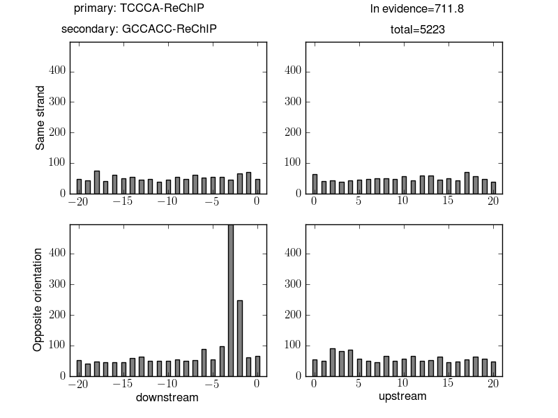
Here we can see that instances of the pair of motifs TCCCA-ReChIP and GCCACC-ReChIP occurred 5,223 times at a distance of less than 20 base pairs. There is an obvious enrichment where an instance of the reverse complement of GCCACC-ReChIP is 2 or 3 base pairs before an instance of TCCCA-ReChIP. Given the 5,223 pairs of instances of these motifs the log evidence in favour of an enriched distribution is large: 711.8.
Given that you have identified a pair of motifs that have some enriched spacing, you may wish to locate instances of the motifs at this spacing. STEME provides a script to do just this:
steme-find-spacings <spacing definitions file>
The spacing definitions file should contain a list of spacings that you are interested in. For example:
TCCCA-ReChIP GCCACC-ReChIP C D 2
TCCCA-ReChIP GCCACC-ReChIP C D 3
would find reverse complemented (C) instances of GCCACC-ReChIP 2 or 3 base pairs downstream (D) of TCCCA-ReChIP instances.
If you have the rpy2 python package and the glmnet, Matrix, plyr and ROCR R packages installed, you can compare the results of two scans to determine which motif instances best discriminate the sets of sequences. The command:
steme-scans-discriminate <sequence statistics 1> <sequence statistics 2>
will fit a lasso model using glmnet to the predicted binding sites and report which motifs are selected by the model. These motifs are the motifs that discriminate best between the two sequence sets. The model fitting uses cross-validation to select a value of lambda (note this is a different lambda than the lambda described above in the STEME scanning model). The output directory will contain a plot demonstrating what AUC was achieved by this lambda:
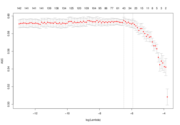
The optimal lambda is shown by the vertical dotted line on the left and a lambda which is within one standard error of the minimum is shown by the vertical dotted line on the right. This lambda.1se is the value used by the lasso.
The ROC curve for the performance of the lasso classifier on the training data is also generated:

The program output will show the coefficients for the motifs in the lasso:
2013-11-27 08:29:35,105 - INFO - Loading statistics from: scan-vertebrate-ac.csv
2013-11-27 08:29:44,478 - INFO - Loading statistics from: scan-vertebrate-noac.csv
2013-11-27 08:29:48,386 - INFO - Joining data
2013-11-27 08:30:00,016 - INFO - Have 2169 motifs
2013-11-27 08:30:00,017 - INFO - Have 5906 sequences
2013-11-27 08:30:00,115 - INFO - 4.6% entries of X are non-zero
2013-11-27 08:30:00,201 - INFO - Creating responses
2013-11-27 08:30:00,204 - INFO - Cross-validating Lasso GLM
2013-11-27 08:30:09,442 - INFO - Evaluating model
2013-11-27 08:30:09,500 - INFO - AUC=0.599042
2013-11-27 08:30:09,506 - INFO - Examine coefficients
2013-11-27 08:30:09,513 - INFO - Using 19 / 2169 motifs
2013-11-27 08:30:09,513 - INFO - beta: -0.871 : (Intercept)
2013-11-27 08:30:09,513 - INFO - beta:  0.006 : E.V.NKX32_06.
2013-11-27 08:30:09,513 - INFO - beta:  0.011 : E.V.GLI3_Q5_01.
2013-11-27 08:30:09,513 - INFO - beta:  0.014 : E.V.OCT4_02.
2013-11-27 08:30:09,514 - INFO - beta:  0.015 : E.V.SNAI2_01.
2013-11-27 08:30:09,514 - INFO - beta:  0.016 : E.V.ASCL2_05.
2013-11-27 08:30:09,514 - INFO - beta:  0.023 : E.V.ESRRA_03.
2013-11-27 08:30:09,514 - INFO - beta:  0.036 : E.V.MAZ_Q6_01.
2013-11-27 08:30:09,514 - INFO - beta:  0.052 : E.V.POU3F2_05.
2013-11-27 08:30:09,514 - INFO - beta:  0.100 : E.V.SOX17_01.
2013-11-27 08:30:09,514 - INFO - beta:  0.118 : E.V.POU5F1B_01.
2013-11-27 08:30:09,514 - INFO - beta:  0.121 : E.V.FIGLA_01.
2013-11-27 08:30:09,514 - INFO - beta:  0.133 : E.V.ZIC3_07.
2013-11-27 08:30:09,514 - INFO - beta:  0.148 : E.V.ISX_04.
2013-11-27 08:30:09,514 - INFO - beta:  0.196 : E.V.OCT4_01.
2013-11-27 08:30:09,514 - INFO - beta:  0.205 : E.V.SOX2_01.
2013-11-27 08:30:09,514 - INFO - beta:  0.228 : E.V.CACD_01.
2013-11-27 08:30:09,514 - INFO - beta:  0.260 : E.V.TCF3_06.
2013-11-27 08:30:09,514 - INFO - beta:  0.292 : E.V.ING4_01.
2013-11-27 08:30:09,514 - INFO - beta:  0.359 : E.V.E2F3_Q6.
2013-11-27 08:30:09,515 - INFO - Saving R workspace
This output shows that the most important motfs in the lasso were E2F3, ING4, TCF3 and CACD and that in total 19 motifs were used out of a possible 2,169.
It is possible to run an elastic-net regularization instead of a lasso by using the --alpha argument to the script. Please see the glmnet documentation for more details.
If you wish to constrain the regression coefficients to positive values you can use --lower-limits=0 as an argument to the script. This can be useful when you are interested in discriminating using motifs that occur in only one of the scans. The example above was run with this argument, hence all the coefficients are positive. Note also that glmnet tends to be much faster when constrained in this way.