Tutorial
Welcome to Kiwi!
Kiwi is a visualization tool that combines geneset analysis (GSA) and a biological network that describes the interactions among genesets to provide an uncluttered view of prominent genesets in a given condition and their relatedness.
Note
A Kiwi run is as easy as a single command-line call:
> python -c "import kiwi; kiwi.plot(gsn='path/to/geneset-geneset-interaction.txt', gss='path/to/geneset-analysis-results.txt')"
In this tutorial, you re-analyze gene expression data for a lung adenocarcinoma vs. normal adjacent tissue comparison from Gatto et al. (2014).
The goal - Why Kiwi?
A limitation of geneset analysis (GSA) stands in the loss of information about the relatedness of genesets.
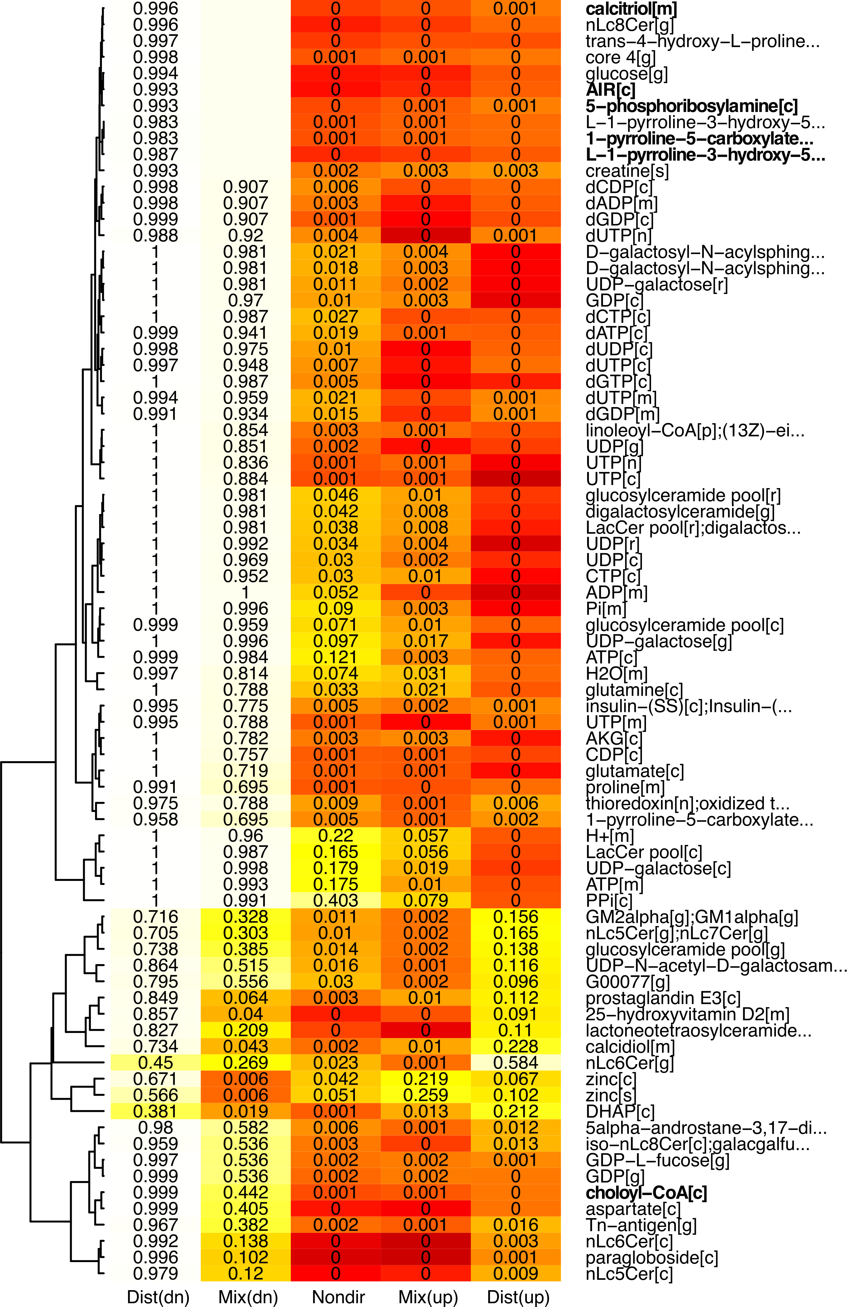
Often, genesets represent biological entities that talk to each other in interaction networks. For example, when a metabolite is defined as a geneset, a typical GSA will output a list of metabolites that are significant as genesets, i.e. most genes that encode for neighboring reactions are differentially expressed in case vs. control. In our example scenario, a GSA run using piano produces the following (trimmed) figure:

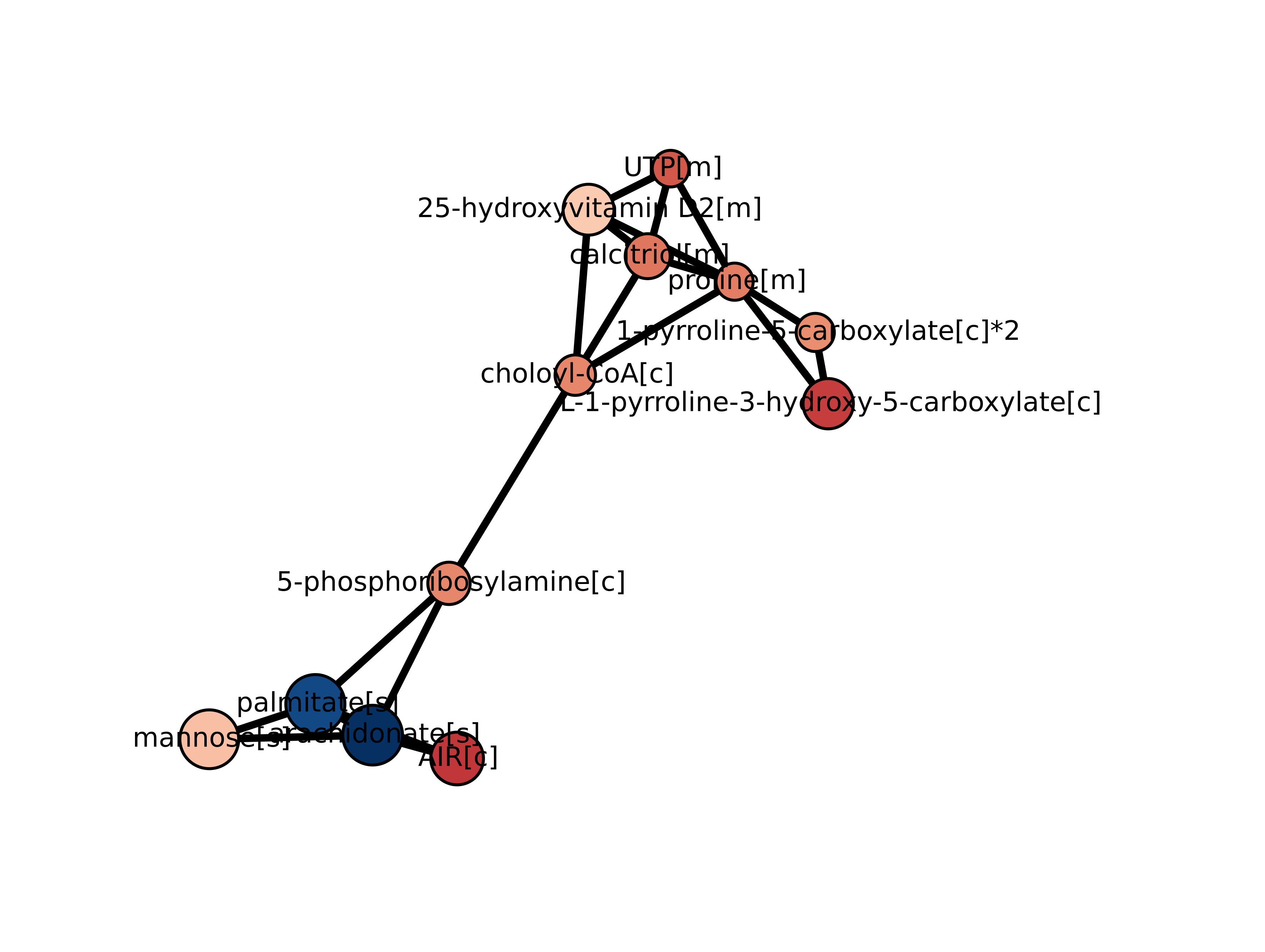
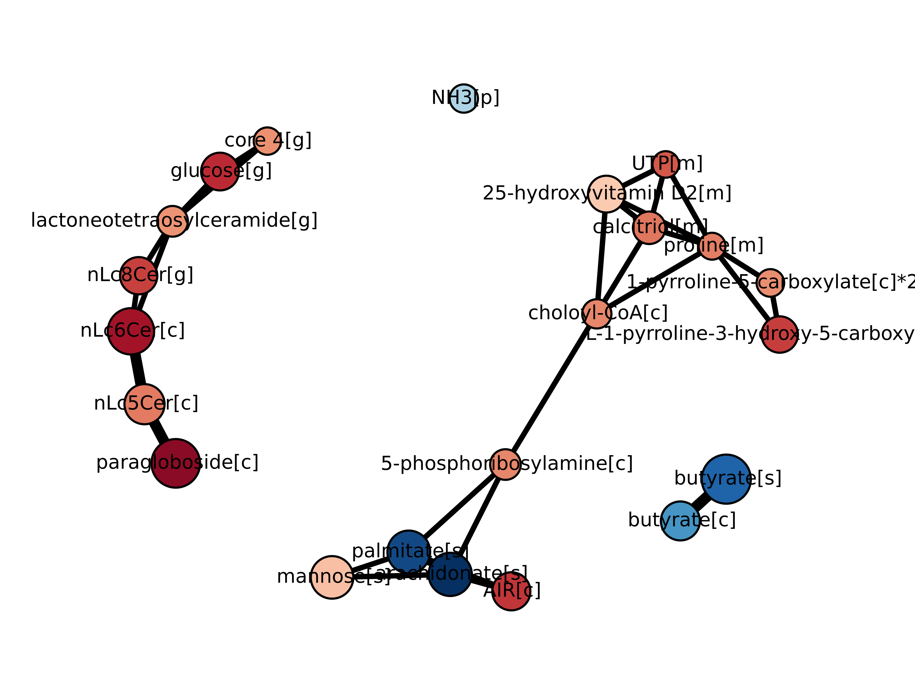
However, metabolites are biologically connected entities by reactions. In the example above, it may be hard to know that chondroitin and heparan sulfates, all of which are significantly regulated in our case, are actually closely connected metabolites, unless you are an expert of glycosaminoglycan biology. A Kiwi run of these GSA results will provide you this missing piece of information:

Preparing the data
Input file requirements
To run Kiwi, the following data files are required:
- A geneset-geneset interaction file (here on referred to as GSN file);
- A geneset statistics result file (here on referred to as GSS file).
Warning
If either the GSN or GSS files are missing or cannot be accessed, Kiwi will halt execution and produce an error.
For a full experience, the following files are also recommended:
- A gene level statistics file (here on referred to as GLS file);
- A gene-geneset file (here on referred to as GSC file);
If provided, the GLS file will output a heatmap that shows which genes contributed to the significance of a geneset.
Available input files
In the subdirectory kiwi/data, there are GSN and GSC for metabolite-metabolite and gene-metabolite (respectively) extracted from genome-scale metabolic models of the following organisms:
- Homo sapiens, from the model HMR2.0
- Mus musculus, from the model MMR
- Saccharomyces cerevisiae, from the model Yeast 7
An example on how these files look like is provided below, in Input file format.
Demo input files
For our example, all input files can be found in the subdirectory kiwi/demo. If you do not have this directory you can download the source from Python Package Index (PyPI), unpack it and find the /demo directory inside.
Input file format
Input files must be tab delimited text files.
The GSN file is a 2 column table where each row contains two interacting genesets, each one per column, with no header. In our example, the GSN file looks like this:
ethanol[c]      acetaldehyde[c]
ethanol[c]      H+[c]
ethanol[c]      NADH[c]
The GSS file is, in its minimum implementation, a two or more column table where each row must contain as first column the genesets and in any column a statistics value for its significance.The header must identify the first column as Name and the geneset statistics column as p-value. It could be as simple as this:
Name    p-value
ethanol[c]      0.0001
acetaldehyde[c] 0.8711
H+[c]   0.2305
NADH[c] 0.0024
The GLS file is, in principle, the same you used to run GSA in the first place. It is a three column table with gene - p*value - fold-change in each row. The genes must be as first column, while *p values and fold-changes must be identified in the headers as p-value and FC, like this:
Gene    p-value FC
ENSG00000000003 1.67109001147722e-48    -1
ENSG00000000005 5.22386360495439e-18    -1
ENSG00000000419 0.153340392968948       -1
The GSC file is, in principle, the same you used to run GSA in the first place. It is a two column table with genesets - genes associations in each row and no header, like this:
ethanol[c]      ENSG00000147576
ethanol[c]      ENSG00000172955
ethanol[c]      ENSG00000180011
Note
Kiwi is optimized to work with results generated using piano . The GSS, GLS, and GSC files can be automatically generated within piano using the function writeFilesForKiwi.R.
Warning
In the current implementation, Kiwi is sensitive to the header content of GSS files. A wrong header will not produce errors while reading the GSS file, but it will most likely cause errors later in the code or generate meaningless results.
Running Kiwi
Once the files are ready, Kiwi can be run with a single command. Go to the Python interpreter and type:
> import kiwi
> kiwi.plot(gsn='path/to/geneset-geneset-interaction.txt', gss='path/to/geneset-analysis-results.txt',
            gls='path/to/gene-level-statistics.txt', gsc='path/to/gene-geneset.txt')
For our example, if your current directory is the module root directory, the call is:
> kiwi.plot(gsn='demo/GSN.txt', gss='demo/GSS_LUAD.txt', gls='demo/GLS_LUAD.txt', gsc='demo/GSC_LUAD.txt')
The following figures are then displayed in your default device:


You are done! Now it is time for the interpretation of results.
Understanding the results
Genesets
When a geneset is deemed significant, it means that the underlying process/function/entity is prominent for the case compared to control. In our example, 1-pyrroline-5-carboxylate is relevant in lung adenocarcinoma compared to tumor-adjacent normal tissue. In those scenarios where extensive regulation is taking place, like in a comparison tumor vs. normal, it is often the case that many genes in a geneset are differentially expressed, yet a GSA run declares the geneset not significant. In our example, a geneset on this line is glutamate-5-semialdehyde (even if it lies just upstream of 1-pyrroline-5-carboxylate). This is due to the extensive background regulation in case vs. control: such genesets may happen to contain a lot of regulated genes just by chance, and a GSA controls for this possibility by correcting the background distribution. The bottom-line is that the genesets shown by Kiwi in the network plot are prominent for your case beyond chance (within a confidence interval of 95%, by default).
If a GLS file is provided, the heatmap shows all genes that contributed to the prominence of each geneset in the network plot. This plot is useful mainly for two reasons:
- It shows the overlap between genesets, i.e. the genes shared by different genesets. Similar genesets cluster together.
- It shows the overlap between genes, i.e. genes that tend to co-express to yield prominence in a geneset.
In general, all these results should be easily interpreted by users familiar with GSA (and most of this information is available in GSA modules).
Interactions
The unicity of a network plot generated by Kiwi stands in the presence of interactions between genesets. These are derived from the geneset-geneset interaction network file. An edge between two genesets indicate that the two are somehow biologically related, and the strength of the relatedness is represented by the edge width.
This information enhances the interpretability of a typical GSA output. In our example, a geneset is a metabolite, and metabolites are interacting with each other via reactions, hence the emergence of metabolic networks. Two metabolites might be prominent as genesets due to strong regulation in very different genes, and yet be related due to vicinity in the metabolic network. The vicinity is measured in terms of shortest path length in the network between two metabolites, i.e. the number of reactions the two metabolites are apart.
In our case vs. control study, 1-pyrroline-5-carboxylate and 5-phosphoribosylamine are prominent genesets because of regulation of different genes, yet they couple proline and pirimidine biosynthesis (i.e. they are not distant in the metabolic network due to the intermediation of choloyl-CoA).
What next?
If you are not satisfied with the presentation of the results (the plot can be cluttered and messy in case of extensive geneset regulation) or the plots provide either too much or too little information, Kiwi offers a number of options and settings that can be tweaked (e.g. the cutoff for the shortest path length or geneset).
There are three ways you could top your experience with Kiwi:
- Export the network in the plot as a GraphML file and import it in Cytoscape. In Cytoscape, the network layout can be controlled in a more flexible way. Moreover, nodes and edges preserve their attributes (significance, directionality index, width, and shortest path length), that can be used in the VizMapper.
- Read the Reference manual. You will find more information on arguments and how plots are created.
- Contribute! Kiwi is open source. You can read the API Documentation, or send your suggestions or bugs to the developers.
