Note: This method computes everything by hand, step by step. For most people, the new API for fuzzy systems will be preferable. The same problem is solved with the new API in this example.
The ‘tipping problem’ is commonly used to illustrate the power of fuzzy logic principles to generate complex behavior from a compact, intuitive set of expert rules.
A number of variables play into the decision about how much to tip while dining. Consider two of them:
quality : Quality of the foodservice : Quality of the serviceThe output variable is simply the tip amount, in percentage points:
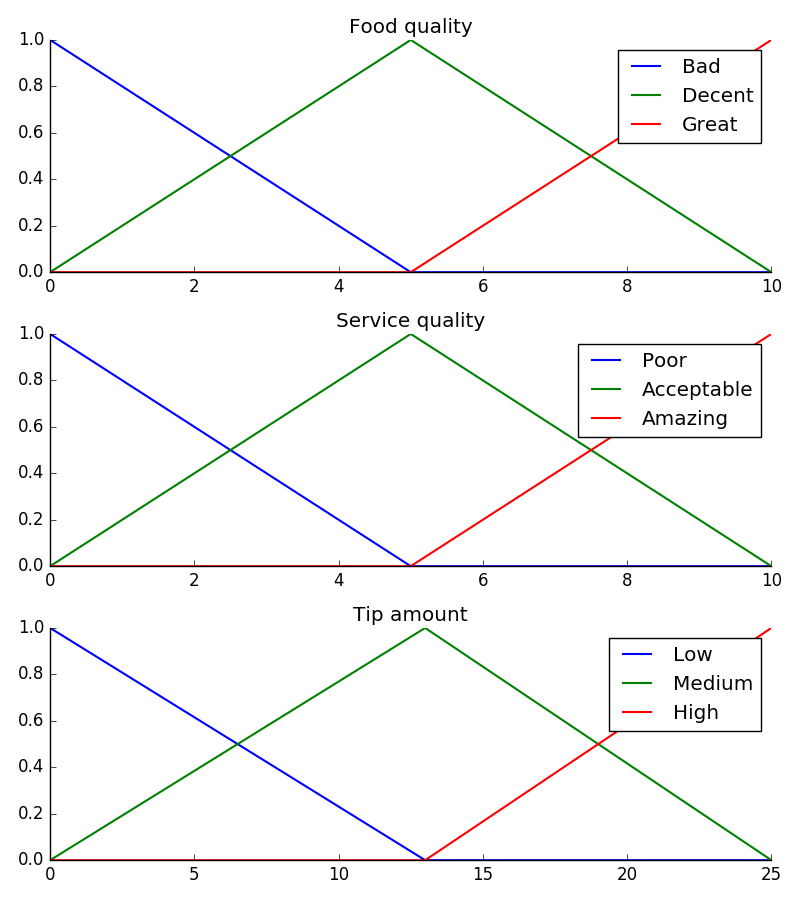
tip : Percent of bill to add as tipFor the purposes of discussion, let’s say we need ‘high’, ‘medium’, and ‘low’ membership functions for both input variables and our output variable. These are defined in scikit-fuzzy as follows
import numpy as np
import skfuzzy as fuzz
import matplotlib.pyplot as plt

# Generate universe variables
#   * Quality and service on subjective ranges [0, 10]
#   * Tip has a range of [0, 25] in units of percentage points
x_qual = np.arange(0, 11, 1)
x_serv = np.arange(0, 11, 1)
x_tip  = np.arange(0, 26, 1)

# Generate fuzzy membership functions
qual_lo = fuzz.trimf(x_qual, [0, 0, 5])
qual_md = fuzz.trimf(x_qual, [0, 5, 10])
qual_hi = fuzz.trimf(x_qual, [5, 10, 10])
serv_lo = fuzz.trimf(x_serv, [0, 0, 5])
serv_md = fuzz.trimf(x_serv, [0, 5, 10])
serv_hi = fuzz.trimf(x_serv, [5, 10, 10])
tip_lo = fuzz.trimf(x_tip, [0, 0, 13])
tip_md = fuzz.trimf(x_tip, [0, 13, 25])
tip_hi = fuzz.trimf(x_tip, [13, 25, 25])

# Visualize these universes and membership functions
fig, (ax0, ax1, ax2) = plt.subplots(nrows=3, figsize=(8, 9))

ax0.plot(x_qual, qual_lo, 'b', linewidth=1.5, label='Bad')
ax0.plot(x_qual, qual_md, 'g', linewidth=1.5, label='Decent')
ax0.plot(x_qual, qual_hi, 'r', linewidth=1.5, label='Great')
ax0.set_title('Food quality')
ax0.legend()

ax1.plot(x_serv, serv_lo, 'b', linewidth=1.5, label='Poor')
ax1.plot(x_serv, serv_md, 'g', linewidth=1.5, label='Acceptable')
ax1.plot(x_serv, serv_hi, 'r', linewidth=1.5, label='Amazing')
ax1.set_title('Service quality')
ax1.legend()

ax2.plot(x_tip, tip_lo, 'b', linewidth=1.5, label='Low')
ax2.plot(x_tip, tip_md, 'g', linewidth=1.5, label='Medium')
ax2.plot(x_tip, tip_hi, 'r', linewidth=1.5, label='High')
ax2.set_title('Tip amount')
ax2.legend()

# Turn off top/right axes
for ax in (ax0, ax1, ax2):
    ax.spines['top'].set_visible(False)
    ax.spines['right'].set_visible(False)
    ax.get_xaxis().tick_bottom()
    ax.get_yaxis().tick_left()

plt.tight_layout()
Now, to make these triangles useful, we define the fuzzy relationship between input and output variables. For the purposes of our example, consider three simple rules:
Most people would agree on these rules, but the rules are fuzzy. Mapping the imprecise rules into a defined, actionable tip is a challenge. This is the kind of task at which fuzzy logic excels.
What would the tip be in the following circumstance:
# We need the activation of our fuzzy membership functions at these values.
# The exact values 6.5 and 9.8 do not exist on our universes...
# This is what fuzz.interp_membership exists for!
qual_level_lo = fuzz.interp_membership(x_qual, qual_lo, 6.5)
qual_level_md = fuzz.interp_membership(x_qual, qual_md, 6.5)
qual_level_hi = fuzz.interp_membership(x_qual, qual_hi, 6.5)
serv_level_lo = fuzz.interp_membership(x_serv, serv_lo, 9.8)
serv_level_md = fuzz.interp_membership(x_serv, serv_md, 9.8)
serv_level_hi = fuzz.interp_membership(x_serv, serv_hi, 9.8)
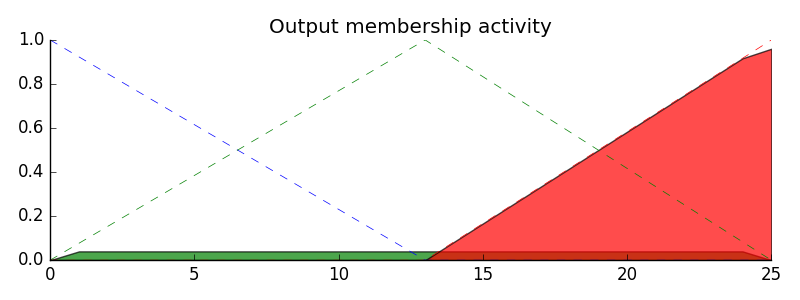
# Now we take our rules and apply them. Rule 1 concerns bad food OR service.
# The OR operator means we take the maximum of these two.
active_rule1 = np.fmax(qual_level_lo, serv_level_lo)
# Now we apply this by clipping the top off the corresponding output
# membership function with `np.fmin`
tip_activation_lo = np.fmin(active_rule1, tip_lo) # removed entirely to 0
# For rule 2 we connect acceptable service to medium tipping
tip_activation_md = np.fmin(serv_level_md, tip_md)
# For rule 3 we connect high service OR high food with high tipping
active_rule3 = np.fmax(qual_level_hi, serv_level_hi)
tip_activation_hi = np.fmin(active_rule3, tip_hi)
tip0 = np.zeros_like(x_tip)
# Visualize this
fig, ax0 = plt.subplots(figsize=(8, 3))
ax0.fill_between(x_tip, tip0, tip_activation_lo, facecolor='b', alpha=0.7)
ax0.plot(x_tip, tip_lo, 'b', linewidth=0.5, linestyle='--', )
ax0.fill_between(x_tip, tip0, tip_activation_md, facecolor='g', alpha=0.7)
ax0.plot(x_tip, tip_md, 'g', linewidth=0.5, linestyle='--')
ax0.fill_between(x_tip, tip0, tip_activation_hi, facecolor='r', alpha=0.7)
ax0.plot(x_tip, tip_hi, 'r', linewidth=0.5, linestyle='--')
ax0.set_title('Output membership activity')
# Turn off top/right axes
for ax in (ax0,):
ax.spines['top'].set_visible(False)
ax.spines['right'].set_visible(False)
ax.get_xaxis().tick_bottom()
ax.get_yaxis().tick_left()
plt.tight_layout()
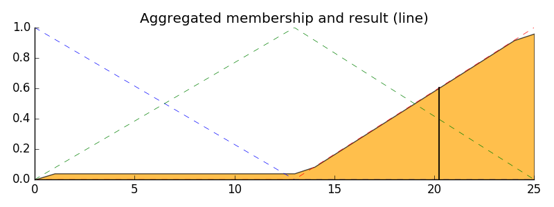
With the activity of each output membership function known, all output membership functions must be combined. This is typically done using a maximum operator. This step is also known as aggregation.
Finally, to get a real world answer, we return to crisp logic from the world of fuzzy membership functions. For the purposes of this example the centroid method will be used.
# Aggregate all three output membership functions together
aggregated = np.fmax(tip_activation_lo,
                     np.fmax(tip_activation_md, tip_activation_hi))

# Calculate defuzzified result
tip = fuzz.defuzz(x_tip, aggregated, 'centroid')
tip_activation = fuzz.interp_membership(x_tip, aggregated, tip)  # for plot

# Visualize this
fig, ax0 = plt.subplots(figsize=(8, 3))

ax0.plot(x_tip, tip_lo, 'b', linewidth=0.5, linestyle='--', )
ax0.plot(x_tip, tip_md, 'g', linewidth=0.5, linestyle='--')
ax0.plot(x_tip, tip_hi, 'r', linewidth=0.5, linestyle='--')
ax0.fill_between(x_tip, tip0, aggregated, facecolor='Orange', alpha=0.7)
ax0.plot([tip, tip], [0, tip_activation], 'k', linewidth=1.5, alpha=0.9)
ax0.set_title('Aggregated membership and result (line)')

# Turn off top/right axes
for ax in (ax0,):
    ax.spines['top'].set_visible(False)
    ax.spines['right'].set_visible(False)
    ax.get_xaxis().tick_bottom()
    ax.get_yaxis().tick_left()

plt.tight_layout()
The power of fuzzy systems is allowing complicated, intuitive behavior based
on a sparse system of rules with minimal overhead. Note our membership
function universes were coarse, only defined at the integers, but
fuzz.interp_membership allowed the effective resolution to increase on
demand. This system can respond to arbitrarily small changes in inputs,
and the processing burden is minimal.
Python source code: download
(generated using skimage 0.2)
 Source