Single Zone Solvers¶

The single zone solvers calculate ionization and/or temperature equilibrium in situations where the densities and temperature can be characterized by single values. Three classes are used to handle three types of equilibrium,

Solve_CE:: Collisional Ionization Equilibrium. Finds ionization fractions at a fixed temperature such that collisional ionizations balance recombinations.
Solve_PCE:: Photo Collisional Ionization Equilibrium. Finds ionization fractions at a fixed temperature such that photo and collisional ionizations balance recombinations.
Solve_PCTE:: Photo Collisional Thermal Equilibrium. Finds ionization fractions and temperatures such that photo and collisional ionizations balance recombinations and heating balances cooling.

More preceisely, the single zone solvers find ionization fractions and/or temperatures that satisfy the following set of equations,

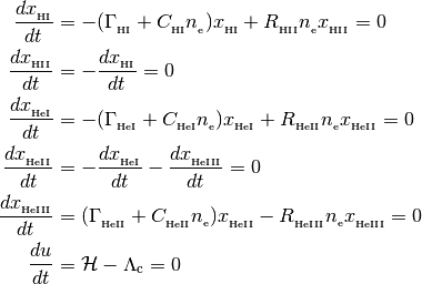
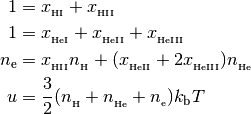
$\frac{dx_{\rm _{HI}}}{dt} &= - (\Gamma_{\rm _{HI}} + C_{\rm _{HI}} n_{\rm _e}) x_{\rm _{HI}} + R_{\rm _{HII}} n_{\rm _e} x_{\rm _{HII}} = 0 \\ \frac{dx_{\rm _{HII}}}{dt} &= - \frac{dx_{\rm _{HI}}}{dt} = 0 \\ \frac{dx_{\rm _{HeI}}}{dt} &= - (\Gamma_{\rm _{HeI}} + C_{\rm _{HeI}} n_{\rm _e}) x_{\rm _{HeI}} + R_{\rm _{HeII}} n_{\rm _e} x_{\rm _{HeII}} = 0 \\ \frac{dx_{\rm _{HeII}}}{dt} &= -\frac{dx_{\rm _{HeI}}}{dt} - \frac{dx_{\rm _{HeIII}}}{dt} = 0 \\ \frac{dx_{\rm _{HeIII}}}{dt} &= (\Gamma_{\rm _{HeII}} + C_{\rm _{HeII}} n_{\rm _e}) x_{\rm _{HeII}} - R_{\rm _{HeIII}} n_{\rm _e} x_{\rm _{HeIII}} = 0 \\ \frac{du}{dt} &= \mathcal{H} - \Lambda_{\rm c} = 0$

with the following closure relationships

$1 &= x_{\rm _{HI}} + x_{\rm _{HII}} \\ 1 &= x_{\rm _{HeI}} + x_{\rm _{HeII}} + x_{\rm _{HeIII}} \\ n_{\rm e} &= x_{\rm _{HII}} n_{\rm _{H}} + ( x_{\rm _{HeII}} + 2 x_{\rm _{HeIII}} ) n_{\rm _{He}} \\ u &= \frac{3}{2} ( n_{\rm _H} + n_{\rm _{He}} + n_{\rm _e} ) k_{\rm b} T$

In the equations above, the $\Gamma_{\rm _X}$ are photoionization rates, the $C_{\rm _X}$ are collisional ionization rates, the $R_{\rm _X}$ are recombination rates, $u$ is the internal energy, $\mathcal{H}$ is the heating function, and $\Lambda_{\rm c}$ is the cooling function.

Collisional Ionization Equilibrium¶

The Solve_CE class assumes a fixed temperature and that all photoionization rates are zero. In this case, there is an analytic solution to the above equations which depends only on the collisional ionization and recombination rates at a given temperature. The following example will produce a solution for 4 temperatures and will use case A rates for each solution (although the case A fraction arguments can also be arrays).

import numpy as np
import rabacus as ra
N = 4
T = 10**np.linspace( 4.0, 5.0, N ) * ra.u.K
fcA_H2 = 1.0; fcA_He2 = 1.0; fcA_He3 = 1.0
kchem = ra.ChemistryRates( T, fcA_H2, fcA_He2, fcA_He3 )
x_ce = ra.Solve_CE( kchem )

The object x_ce now contains ionization fractions for neutral and ionized hydrogen at the four input temperatures,

print x_ce.H1

[  9.97918208e-01   3.73423460e-02   2.86333499e-04   1.71296398e-05] dimensionless

print x_ce.H2

[ 0.00208179  0.96265765  0.99971367  0.99998287] dimensionless

and ionization fractions for neutral, singly ionized, and doubly ionized helium at the same temperatures,

print x_ce.He1

[  9.99999998e-01   9.78969652e-01   1.44418832e-02   1.60194516e-04] dimensionless

print x_ce.He2

[  1.77227599e-09   2.10303478e-02   9.83482722e-01   1.13874960e-01] dimensionless

print x_ce.He3

[  1.84382466e-34   2.68487133e-12   2.07539496e-03   8.85964845e-01] dimensionless

Photo Collisional Ionization Equilibrium¶

The Solve_PCE class assumes that the temperature is fixed but includes non-zero photoionization rates. These solutions depend on the density of hydrogen and helium as well as temperature. In order to make the solvers aware of photoionization rates they need to be included as arguments in the chemistry rates object. The following example will get photoionization rates from the Haardt and Madau 2012 model and use them to solve for photo collisional equilibrium at 4 density-temperature pairs using case B recombination rates.

import numpy as np
import rabacus as ra
N = 4

Yp = 0.24
nH = np.ones(N) * 1.0e-3 / ra.u.cm**3
nHe = nH * 0.25 * Yp / (1-Yp)

pt = ra.HM12_Photorates_Table()
z = 3.0

H1i = np.ones(N) * pt.H1i(z)
He1i = np.ones(N) * pt.He1i(z)
He2i = np.ones(N) * pt.He2i(z)

T = 10**np.linspace( 4.0, 5.0, N ) * ra.u.K
fcA_H2 = 0.0; fcA_He2 = 0.0; fcA_He3 = 0.0

kchem = ra.ChemistryRates( T, fcA_H2, fcA_He2, fcA_He3,
                           H1i=H1i, He1i=He1i, He2i=He2i )

x_pce = ra.Solve_PCE( nH, nHe, kchem )

In the above example we have made the densities and photoionization rates equal for all four temperatures, but this is not necessary (i.e. each element of those arrays can have a different value). The object x_pce now contains ionization fractions for neutral and ionized hydrogen at the four input temperatures,

print x_pce.H1

[ 3.54508432e-04   1.82664733e-04   5.51303759e-05   6.31418283e-06] dimensionless

print x_pce.H2

[ 0.99964549  0.99981734  0.99994487  0.99999369] dimensionless

and ionization fractions for neutral, singly ionized, and doubly ionized helium at the same temperatures,

print x_pce.He1

[ 1.99727141e-04   7.38265776e-05   2.63511233e-05   2.42439604e-05] dimensionless

print x_pce.He2

[ 0.32318511  0.21074971  0.12540601  0.03435841] dimensionless

print x_pce.He3

[ 0.67661516  0.78917647  0.87456764  0.96561735] dimensionless

Photo Collisional Thermal Equilibrium¶

The Solve_PCTE class finds a temperatures and ionization fractions that satisfy the above equations for an array of densities. Because inverse Compton scattering off of CMB photons can be an appreciable cooling mechanism, this class takes a redshift as one of its arguments. The following example will get photoionization and photoheating rates from the Haardt and Madau 2012 model and use them to solve for photo collisional thermal equilibrium at 4 densities. Note that the photoheating rates are attached to the cooling object just as the photoionization rates are attached to the chemistry object. Also note that temperatures are used to initialize the chemistry and cooling objects, but these temperatures will be changed to the equilibrium temperatures during the call to the solver.

import numpy as np
import rabacus as ra
N = 4

Yp = 0.24
nH = 10**np.linspace( -5.0, -1.0, N ) / ra.u.cm**3
nHe = nH * 0.25 * Yp / (1-Yp)

pt = ra.HM12_Photorates_Table()
z = 3.0

H1i = np.ones(N) * pt.H1i(z)
He1i = np.ones(N) * pt.He1i(z)
He2i = np.ones(N) * pt.He2i(z)

H1h = np.ones(N) * pt.H1h(z)
He1h = np.ones(N) * pt.He1h(z)
He2h = np.ones(N) * pt.He2h(z)

T = 10**np.linspace( 4.0, 5.0, N ) * ra.u.K
fcA_H2 = 0.0; fcA_He2 = 0.0; fcA_He3 = 0.0

kchem = ra.ChemistryRates( T, fcA_H2, fcA_He2, fcA_He3,
                           H1i=H1i, He1i=He1i, He2i=He2i )

kcool = ra.CoolingRates( T, fcA_H2, fcA_He2, fcA_He3,
                         H1h=H1h, He1h=He1h, He2h=He2h )

x_pcte = ra.Solve_PCTE( nH, nHe, kchem, kcool, z )

Note

Hubble cooling can be included by passing in the hubble parameter at the desired redshift using the keyword argument Hz. For example

Hz = ra.planck13_cosmology.Hz(z)
x_pcte = ra.Solve_PCTE( nH, nHe, kchem, kcool, z, Hz=Hz )

We have used non-uniform values for both the density and temperature arrays in this example. The particular temperatures used to instantiate the chemistry and cooling objects is not important as this solver will converge to the equilibrium temperatures for the given densities. The returned object x_pcte contains ionization fractions and equilibrium temperatures for the input densities. The ionization fractions for neutral and ionized hydrogen are,

print x_pcte.H1

[  2.19371954e-06   2.40811392e-05   8.76128859e-04   2.65644453e-02] dimensionless

print x_pcte.H2

[ 0.99999781  0.99997592  0.99912387  0.97343555] dimensionless

The ionization fractions for neutral, singly ionized, and doubly ionized helium are,

print x_pcte.He1

[  1.26614727e-08   1.94244006e-06   9.45705638e-04   4.52573115e-02] dimensionless

print x_pcte.He2

[ 0.00311191  0.03711927  0.56211876  0.93000539] dimensionless

print x_pcte.He3

[ 0.99688808  0.96287879  0.43693553  0.0247373 ] dimensionless

and the equilibrium temperatures at the input densities are,

print x_pcte.Teq

[ 17989.27445847  35889.65514996  19901.78191525  12452.52329718] K