The waveform module: Creating and manipulating discrete-time functions

The Waveform class creates, manipulate and plot discrete functions of time.

It was primarily designed to work with the analog input/output functions of the MCCDAQ Python driver usb2600.usb2600, but is much more general in scope.

The Waveform class can do:

• single- and multi-channel waveforms
• time plots
• XY plots
• XYZ plots (both regularly and randomly spaced data)
• Fourier transform
• simple arithmetics (add and multiply waveforms, and waveforms and scalars)

Functions are included to create some usual waveforms:

• sine
• helix
• gosine (connects two points with a sine curve)
• linscan (triangular waveform with rounded edges)

Copyright Guillaume Lepert, 2014

mccdaq.utilities.waveform.timescale = {'week': 604800, 's': 1.0, 'ms': 1000.0, 'min': 0.016666666666666666, 'h': 0.0002777777777777778, 'ns': 1000000000.0, 'year': 31557600.0, 'day': 86400.0, 'us': 1000000.0}

Define time units, relative to the second.

class mccdaq.utilities.waveform.Waveform(data, dt, t0=0, padding=1)

A simple class to create and manipulate waveforms (functions of time).

Parameters:

• data (array-like) – the data
• dt (float) – the waveform sampling interval
• t0 (float) – the waveform time origin (timestamp of first element of data)
• padding (int) – minimum length of the waveform, which will be padded right with 0 if its length is smaller.

pad(padding, value=0)

Right padding.

Parameters:

• padding – the waveform final length
• value – what to pad with

plot(style='')

Plot all waveforms vs time

plotxy(style='', channels=(0, 1))

XY plot for 2D waveforms.

plotxyz(res, channels=(0, 1, 2), interp=u'nn')

Density plot of irregularly spaced data

plot_linear_subset(ch=(0, 1, 2), **kwargs)

Density plot of the linear section of the data, if defined

t()

Calculate and returns the time vector.

fourier(power=True, shift=False)

Calculate the Fourier transform of all waveforms in the object.

Returns a new waveform object where dt is the frequency interval.

mccdaq.utilities.waveform.sine(frequency=1, amplitude=1, offset=0, phase=0, nsamples=100, rate=10, tunit='s')

Return a sine wave.

\(y(t) = DC + A \sin(2 \pi f t + \phi)\)

Parameters:

• frequency – frequency f of the sine wave
• amplitude – amplitude A of the sine wave (peak to average)
• phase – phase \(\phi\) of the sine wave
• offset – DC offset
• nsamples – number of samples in the final waveform
• rate – sampling rate, in Hz
• tunit – time unit to use (see timescale)

Return type:

Waveform

mccdaq.utilities.waveform.helixscan(amplitude, turns)

Returns a two-channel waveform that makes a 2D closed helix pattern.

Parameters:amplitude – scan amplitude Param:turns: number of turns Example:

>>> a = waveform.helixscan(1,10)
>>> a.plotxy()

produces the following scan pattern:

mccdaq.utilities.waveform.gosine(a, b, dt, rate, t0=0)

From A to B in a graceful fashion.

This is done with a cosine arc \(y(t) = a + (b-a) (1-\cos(2 \pi f t))/2\)

Parameters:

• a – starting value
• b – final value
• dt – time interval between a and b
• rate – waveform sampling rate
• t0 – starting time at a

Return type:

Waveform

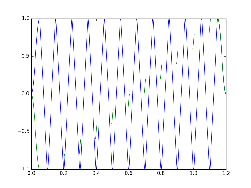
mccdaq.utilities.waveform.linscan(amplitude=1, lines=100, fscan=10, rate=10000, cap=0.08)

Return a two-channel quasi-sinusoidal waveform made of linear segments joined by sine curves.

Parameters:

• amplitude – amplitude of the waveform
• lines – number of periods
• fscan – frequency of the waveform
• rate – sampling rate
• cap – fraction of the waveform spend in the sine cap. between 0 (triangular wave) and 1 (pure sine wave)

Return type:

Waveform

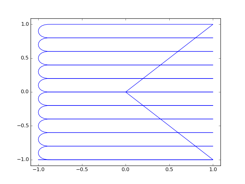
The Waveform.linear_subset attribute of the returned object is set to indicate the linear portions of the waveform (this is useful when using this waveform to drive a usb2600.usb2600.USB2600_Sync_AIO_Scan scan).

Exemple:

>>> a = waveform.linscan(1,10,10,1000,0.08)
>>> a.plot()
>>> a.plotxy()

produces the two-channel waveform shown below. The right figure shows the corresponding 2D scan pattern when the two channel are driving X and Y scanning mirrors (for example).