Tutorial

In this example we will use cyipopt to solve an example problem, number 71 from the Hock-Schittkowsky test suite [1],

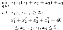
with the starting point,

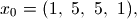
and the optimal solution,

Getting started

Before you can use cyipopt, you have to import it:

import ipopt

Defining the problem

To define the problem we use the ipopt.problem class:

x0 = [1.0, 5.0, 5.0, 1.0]

lb = [1.0, 1.0, 1.0, 1.0]
ub = [5.0, 5.0, 5.0, 5.0]

cl = [25.0, 40.0]
cu = [2.0e19, 40.0]

nlp = ipopt.problem(
            n=len(x0),
            m=len(cl),
            problem_obj=hs071(),
            lb=lb,
            ub=ub,
            cl=cl,
            cu=cu
            )

The constructor of the ipopt.problem class requires n: the number of variables in the problem, m: the number of constraints in the problem, lb and ub: lower and upper bounds on the variables, and cl and cu: lower and upper bounds of the constraints. problem_obj is an object whose methods implement the objective, gradient, constraints, jacobian, and hessian of the problem:

class hs071(object):
    def __init__(self):
        pass

    def objective(self, x):
        #
        # The callback for calculating the objective
        #
        return x[0] * x[3] * np.sum(x[0:3]) + x[2]

    def gradient(self, x):
        #
        # The callback for calculating the gradient
        #
        return np.array([
                    x[0] * x[3] + x[3] * np.sum(x[0:3]),
                    x[0] * x[3],
                    x[0] * x[3] + 1.0,
                    x[0] * np.sum(x[0:3])
                    ])

    def constraints(self, x):
        #
        # The callback for calculating the constraints
        #
        return np.array((np.prod(x), np.dot(x, x)))

    def jacobian(self, x):
        #
        # The callback for calculating the Jacobian
        #
        return np.concatenate((np.prod(x) / x, 2*x))

    def hessianstructure(self):
        #
        # The structure of the Hessian
        # Note:
        # The default hessian structure is of a lower triangular matrix. Therefore
        # this function is redundant. I include it as an example for structure
        # callback.
        #
        global hs

        hs = sps.coo_matrix(np.tril(np.ones((4, 4))))
        return (hs.col, hs.row)

    def hessian(self, x, lagrange, obj_factor):
        #
        # The callback for calculating the Hessian
        #
        H = obj_factor*np.array((
                (2*x[3], 0, 0, 0),
                (x[3],   0, 0, 0),
                (x[3],   0, 0, 0),
                (2*x[0]+x[1]+x[2], x[0], x[0], 0)))

        H += lagrange[0]*np.array((
                (0, 0, 0, 0),
                (x[2]*x[3], 0, 0, 0),
                (x[1]*x[3], x[0]*x[3], 0, 0),
                (x[1]*x[2], x[0]*x[2], x[0]*x[1], 0)))

        H += lagrange[1]*2*np.eye(4)

        #
        # Note:
        #
        #
        return H[hs.row, hs.col]

    def intermediate(
            self,
            alg_mod,
            iter_count,
            obj_value,
            inf_pr,
            inf_du,
            mu,
            d_norm,
            regularization_size,
            alpha_du,
            alpha_pr,
            ls_trials
            ):

        #
        # Example for the use of the intermediate callback.
        #
        print "Objective value at iteration #%d is - %g" % (iter_count, obj_value)

The intermediate() method if defined is called every iteration of the algorithm. The jacobianstructure() and hessianstructure() methods if defined should return a tuple which lists the non zero values of the jacobian and hessian matrices respectively. If not defined then these matrices are assumed to be dense. The jacobian() and hessian() methods should return the non zero values as a falttened array. If the hessianstructure() method is not defined then the hessian() method should return a lower traingular matrix (flattened).

Setting optimization parameters

Setting optimization parameters is done by calling the ipopt.problem.addOption() method, e.g.:

nlp.addOption('mu_strategy', 'adaptive')
nlp.addOption('tol', 1e-7)

The different options and their possible values are described in the ipopt documentation.

Executing the solver

The optimization algorithm is run by calling the ipopt.problem.solve() method, which accepts the starting point for the optimization as its only parameter:

x, info = nlp.solve(x0)

The method returns the optimal solution and an info dictionary that contains the status of the algorithm, the value of the constraints multipliers at the solution, and more.

Where to go from here

Once you feel sufficiently familiar with the basics, feel free to dig into the reference. For more examples, check the test/ subdirectory of the distribution.

[1]	W. Hock and K. Schittkowski. Test examples for nonlinear programming codes. Lecture Notes in Economics and Mathematical Systems, 187, 1981.