
gdsCAD is a simple, but powerful, Python package for creating, reading, and manipulating GDSII layout files. It’s suitable for scripting and interactive use. It excels particularly in generating designs with multiple incrementally adjusted objects. gdsCAD uses matplotlib to visualize everything from individual geometry primitives to the entire layout.
This User’s Guide is intended to get you started with gdsCAD. It will introduce you to the package’s most basic objects, before showing you how to organize and manipulate groups of objects. More advanced devices can be found in the Examples page. Details of the interface, and information for developers can be found in The gdsCAD API pages.
gdsCAD is derived from gdspy by Lucas Heitzmann Gabrielli. The most significant difference is that gdsCAD adds the Layout to allow simultaneous work on multiple GDSII streams, and simplifies the import process. The saving scheme also allows the user to be lazy in maintaining Cell names, and the package is organized into submodules based on function. For its part gdspy has more advanced boolean and fracture functions not yet supported in gdsCAD.
Here is a minimal working script that creates a box and inserts it into a cell which is then added to a layout. The layout is saved as a GDSII stream in the file ‘output.gds’. This illustrates the general gdsCAD workflow of building geometry, adding that to cells, and then adding cells to a layout, before saving. In this example the layout is also displayed in a viewer:
from gdsCAD import *
# Create a Cell and add the box
cell=core.Cell('TOP')
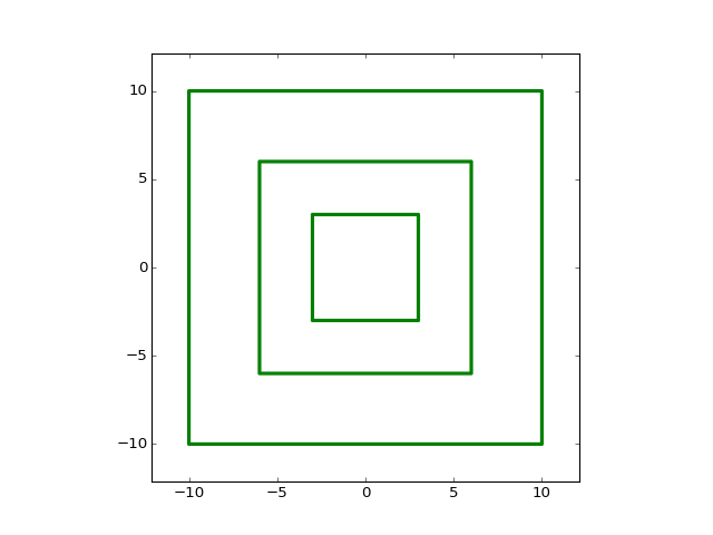
# Create three boxes on layer 2 of different sizes centered at
# the origin and add them to the cell.
for l in (3,6,10):
box=shapes.Box((-l,-l), (l,l), width=0.2, layer=2)
cell.add(box)
# Create a layout and add the cell
layout = core.Layout('LIBRARY')
layout.add(cell)
# Save the layout and then display it on screen
layout.save('output.gds')
layout.show()
(Source code, png, hires.png, pdf)
There are only two basic objects for drawing art in a GDSII file: Boundary and Path. The object Text creates annotations that can be seen in design viewers, but will not print. All the other primitive classes (Cell, Elements, Layout, etc...) are for managing and organizing objects based on Boundary and Path.
Boundary objects are filled, closed polygons. They correspond to the Boundary object defined in the GDSII specification. Boundaries are created by specifying the sequence of points that define the boundary outline. They are closed automatically.
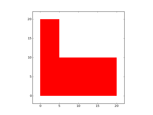
The following code will create an L-shaped polygon:
from gdsCAD import *

points=[(0,0), (20,0), (20,10), (5,10), (5,20), (0,20)]
bdy = core.Boundary(points)
bdy.show()
(Source code, png, hires.png, pdf)
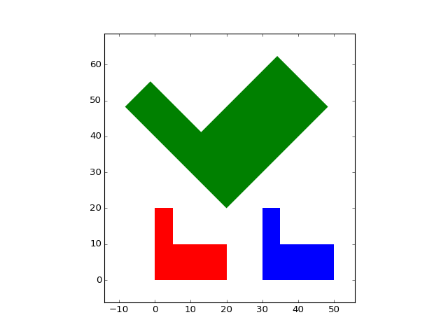
Boundaries can be copied, and subjected to the geometric transformations rotate, reflect, scale, and translate. There are two ways to make transformations to an object, the first is to use the class methods. These will apply the transformation in place, and the methods all return the object itself so it’s easy to chain transformations together. The alternative is to use the transformation functions found in the utils module. These will make a copy of the object and apply the transformation to the copy. These can also can be used on points or lists of points:
# Transform the body using methods
bdy2 = bdy.copy()
bdy2.scale(2).rotate(45).translate((20,20))
bdy2.layer=2     # Change the layer so that we can see it more easily
bdy2.show()

# Transform the body using the transformations in utils
bdy3 = utils.translate(bdy, (30,0))
bdy3.layer = 3
bdy3.show()
(Source code, png, hires.png, pdf)
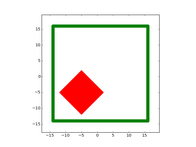
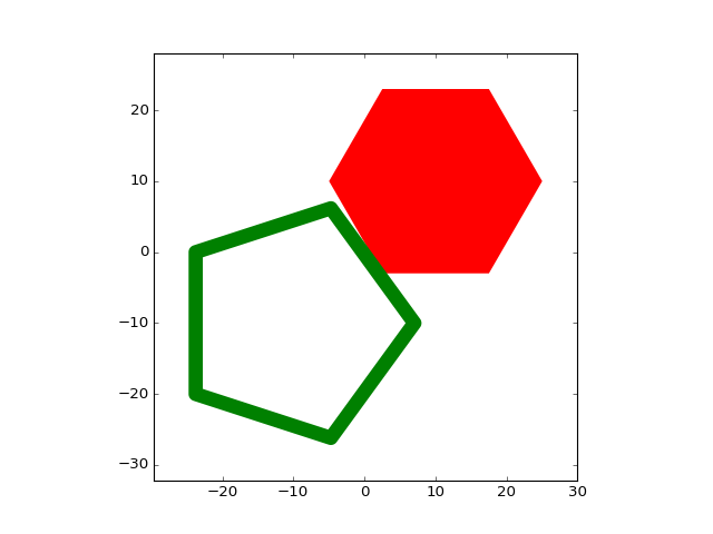
The bounding_box attribute tells you the smallest bounding box which the object can fit within in the form [[minx, miny], [maxx, maxy]]. In the figure below the green line shows the red shape’s bounding box.
(Source code, png, hires.png, pdf)
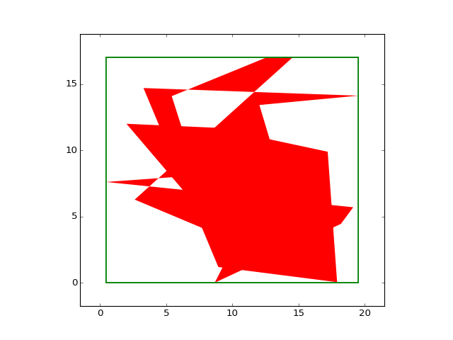
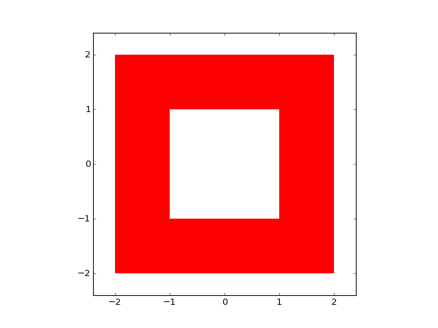
Note that red Boundary shown above is technically illegal, since in the GDSII specification Boundaries cannot be self intersecting, or have internal voids. The way in which such shapes will render is indeterminate. Voids can be created legally, by using XOR postprocessing, or through the use of “keyhole” type geometries:
# Inner box: CCW point order
inner_box = [[1,0], [1,1], [-1,1], [-1,-1], [1,-1], [1,0]]

# Outer box: CW point order
outer_box  = [[2, 0], [2, -2], [-2,-2], [-2, 2], [2,2], [2,0]]

# Join boxes together
points = inner_box + outer_box
bdy = core.Boundary(points)
bdy.show()
(Source code, png, hires.png, pdf)
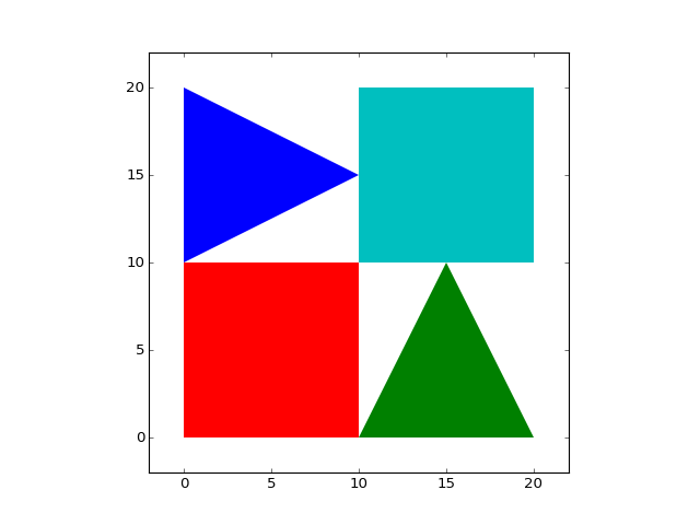
Boundaries, and all other drawing objects, have layer and datatype attributes like GDSII elements. These can be specified as optional keyword arguments when the object is initialized. If absent layer and datatype are assigned values based on core.default_layer and core.default_datatype. Alternatively, they can be adjusted after the object is created by assigning a new value to the obj.layer attribute:
from gdsCAD import *

points=[(0,0), (10,0), (10,10), (0,10)]
bdy = core.Boundary(points)
bdy.show()

points2=[(10,0), (20,0), (15,10)]
bdy2 = core.Boundary(points2, layer=2)
bdy2.show()

points3=[(0,10), (0,20), (10,15)]
bdy3 = core.Boundary(points3)
bdy3.layer = 3
bdy3.show()

core.default_layer=4

points4=[(10,10), (20,10), (20,20), (10,20)]
bdy4 = core.Boundary(points4)
bdy4.show()
(Source code, png, hires.png, pdf)
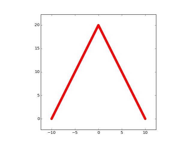
In contrast to a Boundary which is closed and filled, a Path is unfilled and may be open. They are often employed for drawing wires or other fine electrical connections. Paths have a finite width given by third parameter.:
points=[(-10,0), (0,20), (10,0)]
pth = core.Path(points, 0.5)
pth.show()
(Source code, png, hires.png, pdf)
Paths can have different endpoint styles specified by the optional pathtype argument, however because of how they are implement Paths are always shown with rounded endcaps. Thus designs that depend critically on the endpoint geometry should be checked in an external GDSII viewer.
Like Boundaries, Paths cannot legally self intersect.
gdsCAD provides several higher order classes for conveniently creating common objects. These are contained in the module gdsCAD.shape and are derived from the base classes core.Boundary and core.Path.
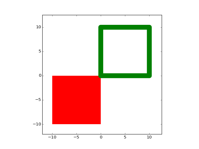
These two classes create filled and unfilled rectangles respectively. The are defined by the positions of two opposite corners, and in the case of Box, the width of the path:
rect=shapes.Rectangle((-10,-10), (0,0))
box=shapes.Box((0,0), (10,10), 1.0, layer=2)
(Source code, png, hires.png, pdf)
Again, they can transformed through simple geometrical transformations:
rect.rotate(45, center=(-5,-5))
box.scale(3).translate((-14,-14))
(Source code, png, hires.png, pdf)
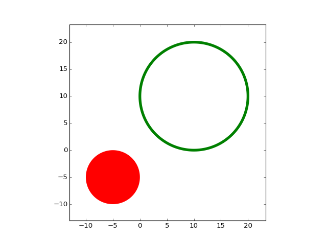
These two classes create filled and unfilled circles. They are defined by their center position and radius:
disk=shapes.Disk((-5,-5), 5)
circ=shapes.Circle((10,10), 10, 0.5, layer=2)
(Source code, png, hires.png, pdf)
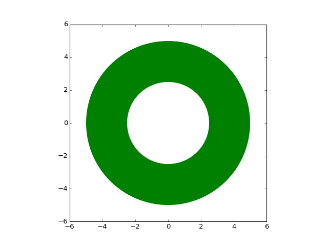
It’s possible to draw a disks with a hollow inner radius, this is constructed using a keyhole geometry so it does not defy the restriction that Boundaries cannot have internal voids:
disk=shapes.Disk((0,0), 5, inner_radius=2.5)
(Source code, png, hires.png, pdf)
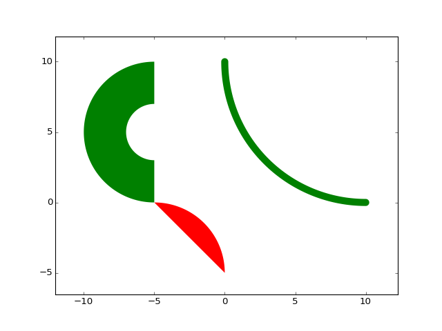
It is possible to draw only segments of both Circles and Disks by specifying an initial and final angle:
disk_arc = shapes.Disk((-5,-5), 5, initial_angle=0, final_angle=90)
circ_segment = shapes.Circle((10,10), 10, 0.5, initial_angle=180, final_angle=270, layer=2)
circ_arc=shapes.Disk((-5, 5), 5, inner_radius = 2, initial_angle=90, final_angle=270, layer=2)
(Source code, png, hires.png, pdf)
The two classes RegPolygon and RegPolyline make filled and unfilled regular polygons respectively. The call signature is much the same as for Disk and Circle, with the addition of a parameter N to specify the number of sides:
hex = shapes.RegPolygon((10,10), 15, 6)
pent = shapes.RegPolyline((-10,-10), 20, 5, 2, layer=2)
(Source code, png, hires.png, pdf)
There are two ways of adding text to a design: core.Text and shapes.Label or shapes.LineLabel.
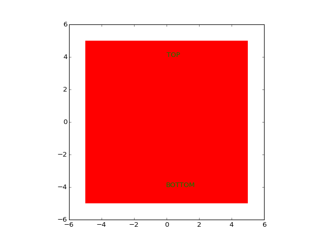
The class Text permits notes and annotations to be added to a design. These will not be printed on the mask are intended only for clarification during the design process. Since they are not true drawing geometry they do not scale in a physical manner with other drawing geometry.
(Source code, png, hires.png, pdf)
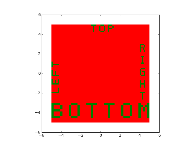
On the other hand, annotations made with Label will print with other mask art. In addition to indicating the layer, string to print, and the position Label, requires a text size in user units.:
top = shapes.Label('TOP', 1, (-1, 4), layer=2)
bottom = shapes.Label('BOTTOM', 2, (-5,-5), layer=2)
left = shapes.Label('LEFT', 1, (-4,-2), angle=90, layer=2)
right = shapes.Label('RIGHT', 1, (4,2), horizontal=False, layer=2)
(Source code, png, hires.png, pdf)
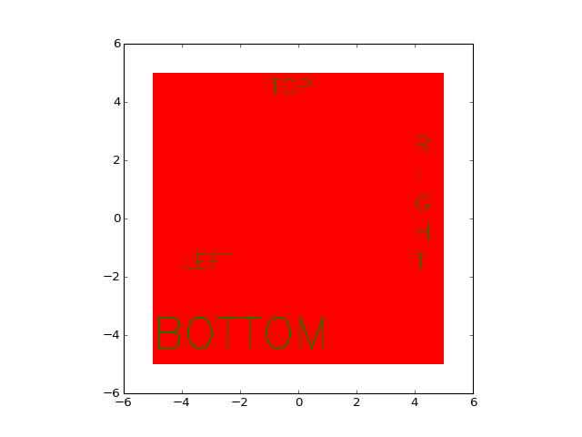
As an alternative way of drawing text, a line based vector font is provided. Internally it is directly based on the Hershey Vector Font so a large variety of fonts and symbols are available. While LineLabel looks nicer in most cases it is not a monospace font and hence not suited for all use cases.
The LineLabel allows mostly the parameters of Vector but no rotation by angle:
top = shapes.LineLabel('TOP', 1, (-1, 4), layer=2)
bottom = shapes.LineLabel('BOTTOM', 2, (-5,-5), layer=2)
left = shapes.LineLabel('LEFT', 1, (-4,-2), horizontal=True, layer=2)
right = shapes.LineLabel('RIGHT', 1, (4,2), horizontal=False, layer=2)
(Source code, png, hires.png, pdf)
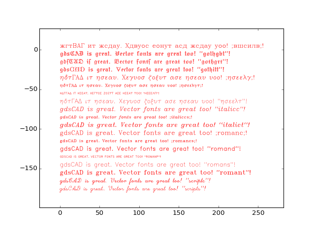
Many other fonts can also be selected. Note the use of add_text to add more text to the `LineLabel`:
FONTS = ['cyrilc', 'gothgbt', 'gothgrt', 'gothitt', 'greekc',
         'greekcs', 'greekp', 'greeks', 'italicc', 'italiccs',
         'italict', 'romanc', 'romancs', 'romand', 'romanp',
         'romans', 'romant', 'scriptc', 'scripts']
TEST_TEXT = 'gdsCAD is great. Vector fonts are great too! "%s"!\n'

label = gdsCAD.shapes.LineLabel('', 10)
for font in FONTS:
    label.add_text(TEST_TEXT % font, font)
(Source code, png, hires.png, pdf)
gdsCAD provides three different schemes for collecting different pieces of artwork together: Elements, Cell, and Layout.
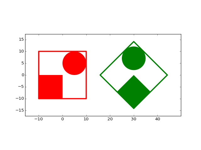
The Elements object is essentially a list of drawing elements. Elements allow groups of objects to be conveniently transformed as one. All elements in the list are coerced to have the same layer, and changing the layer of the Elements object changes the layer of all it’s members:
one = shapes.Box((-10,-10), (10,10), 0.5)
two = shapes.Rectangle((-10,-10), (0,0), layer=2)
three = shapes.Disk((5,5), 5, layer=3)

group = core.Elements((one, two, three))
group.show()

group2 = utils.rotate(group, 45).translate((30,0))
group2.layer = 2
group2.show()
(Source code, png, hires.png, pdf)
There are several different methods for initializaing an Elements. Consult the API reference for more examples.
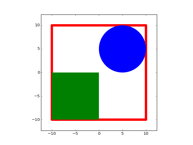
Cells are collections of multiple geometry elements, and references to other Cells. The contents of a Cell can have different datatypes and layers, so they are a good way of grouping together the many elements that make up a device. Every Cell has its own name.
(Source code, png, hires.png, pdf)
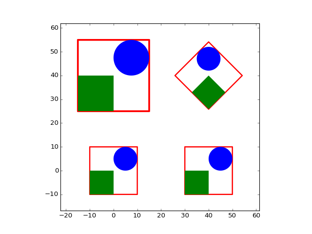
The power of a Cell is that it can itself be inserted as a reference into other Cells. Note that Cells cannot contain circular references. The inserted reference can be subjected to the geometrical transforms, translation (origin), scaling (magnification), and rotation:
top = core.Cell('TOP')

ref1 = core.CellReference(cell)
top.add(ref1)

# Translate
ref2 = core.CellReference(cell, origin=(40,0))
top.add(ref2)

# Scale and Translate
ref3 = core.CellReference(cell, origin=(0, 40), magnification=1.5)
top.add(ref3)

# Rotate and Translate
ref4 = core.CellReference(cell, origin=(40,40), rotation=45)
top.add(ref4)
(Source code, png, hires.png, pdf)
When a Cell is added to another Cell using the .add() method this is done by implicitly creating a CellReference object and adding that. Additional parameters to add are interpreted as parameters to the CellReference initialization.:
# This is shorthand...
myCell.add(anotherCell, origin=(20,10))

# ... for this.
ref = core.CellReference(anotherCell, origin=(20,10))
myCell.add(ref)
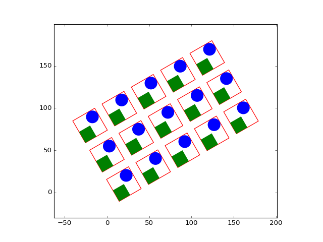
Many references to a``Cell`` arranged on a rectilinear grid can be created with a CellArray. In this case you specify the number of rows and columns for the array, along with a spacing, and optional arguments indicating the magnification, rotation and translation of the array.:
top = core.Cell('TOP')

array = core.CellArray(cell, 5, 3, (40,40), origin=(20,10), rotation=30, magnification=1.5)
top.add(array)
top.show()
(Source code, png, hires.png, pdf)
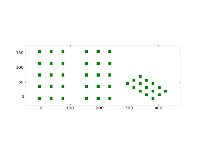
The `spacing` parameter can be either a 2D vector or a pair of 2D vectors. The latter are interpreted as a pair of basis vectors that describe the lattice, and can be used to generate non-orthogonal arrays. The entries of the former give the spacing in the x and y direction for an orthogonal lattice.:
# A square lattice with 40 unit spacing
arr1 = core.CellArray(cell, 3, 5, spacing=(40,40))
top.add(arr1)

# The same specified with a pair of 2D vectors
arr2 = core.CellArray(cell, 3, 5, spacing=((40,0), (0,40)), origin = (160, 0))
top.add(arr2)

# A hexagonal lattice
a=25.
arr3 = core.CellArray(cell, 3, 5, ((a*sqrt(3)/2, a/2), (a*sqrt(3)/2, -a/2)), origin = (300, 50))
top.add(arr3)
(Source code, png, hires.png, pdf)
Note that Cells do not support geometric transformations. So you cannot directly scale or translate a Cell. Instead, apply geometric transforms to a CellReference of the Cell.
The most basic gdsCAD object is the Layout, which is essentially the GDS stream that you will send to the mask shop. A Layout contains many Cells which can in turn contain drawing elements or references to other Cells. Those Cells in a Layout which are not referred to by any other Cell are known as top level Cells:
cell1 = core.Cell('CELL1')

cell2 = core.Cell('CELL2')

# cell2 is a top-level cell, cell1 is not.
cell2.add(cell1)

layout = core.Layout('LAYOUT')

layout.add(cell2)

# This will return a reference to cell2 only
layout.top_level()
The Layout also plays the important role of keeping track of the scale information for the design. Spatial dimensions of objects in gdsCAD have no units, and the size of objects is determined by the units specified in the Layout. Two parameters govern how dimensions are interpreted: units and precision, these can both be adjusted when the library is created. The default is for units to be in um and precision to be in nm. With this unit scheme a 10x10 box would have dimensions when printed of 10um x 10um, and the smallest possible box would be 1nm x 1nm (although that’s very unlikely to print). In practice it’s best to use the defaults and measure everything in um.
Layout is subclassed from the Python dict, so the Cells within a Layout can be accessed by their name like a Python dict, and it is possible to iterate over the names of the cells:
from gdsCAD import *

A=core.Cell('CELL A')
B=core.Cell('CELL B')

l=core.Layout('layout')
l.add(A)
l.add(B)

# Prints information on cell A
print l['CELL A']

# Prints the names of all cells
for name in l:
    print name

# Remove Cell A
del l['CELL A']
A Layout can be saved to a binary GDSII stream by using the method save(fname). It can be displayed using the method show().
GDSII keeps track of the relationships between Cells according to their names, so it’s important that every Cell in a GDS file have a unique name. In contrast gdsCAD keeps track of cell references by using pointers to the Python object, so the Cell name is only a useful label, but not a critical identifier, and it is not essential that Cell names in gdsCAD be unique. When a Layout is saved, any conflicting Cell names are made unique by appending an alphanumeric code.
The following attributes can be found in most (if not all) classes:
Drawing elements contain:
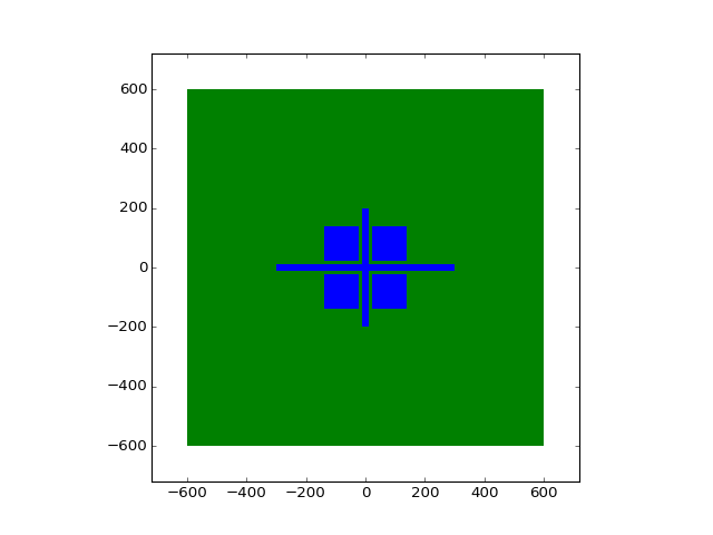
GDSII streams that have been saved to file can be loaded into gdsCAD using the function GdsImport(). This loads the file and returns its contents in the form of a Layout. It handles most, but not all GDSII stream elements. In this example it loads the builtin Layout of alignment marks included with gdsCAD:
amarks = core.GdsImport(mark_file)
amarks.show()
(Source code, png, hires.png, pdf)
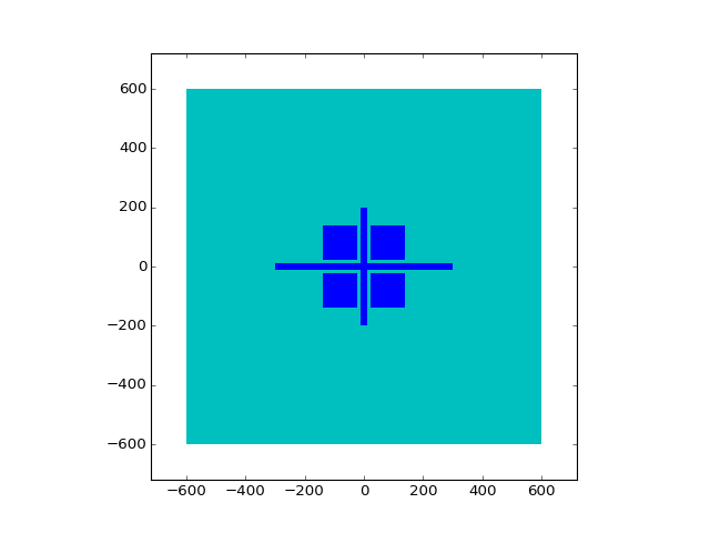
GdsImport accepts several optional arguments that allow the cell names, layers, and datatypes to be reassigned on import. For instance the following will move all the art on layer 2 to layer 4:
amarks = core.GdsImport(mark_file, layers={2:4})
amarks.show()
(Source code, png, hires.png, pdf)