Download the software at http://pypi.python.org/pypi/eq_band_diagram - or submit complaints and corrections at its GitHub page
Written by Steve Byrnes, 2012 (http://sjbyrnes.com)
Software is released under MIT license.
This is a program written in Python / NumPy that calculates equilibrium band structures of planar multilayer semiconductor structures. (It solves the "Poisson-Boltzmann equation" via finite differences.)
"Equilibrium" means "flat fermi level", with V=0 and I=0. This assumption makes the calculation much much simpler. If you look at just the essential algorithm (leaving out my explanations, examples, plots, tests, etc.), it would not even be 50 lines of code.
So this is a relatively simple program for a relatively simple calculation. You can understand how it works, play around with it, etc. But if you're interested in serious, accurate semiconductor simulation, then don't waste your time with this. Get a real TCAD program!
example1(): A p / n junction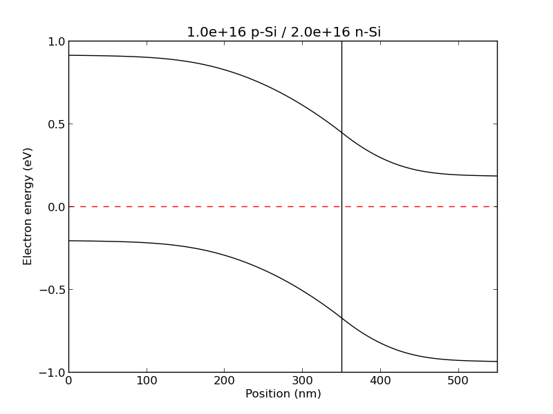
example2(): A n+ / n junction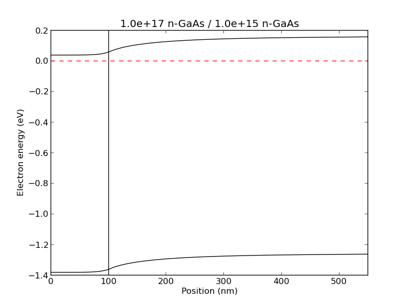
example3(): A bipolar transistor structure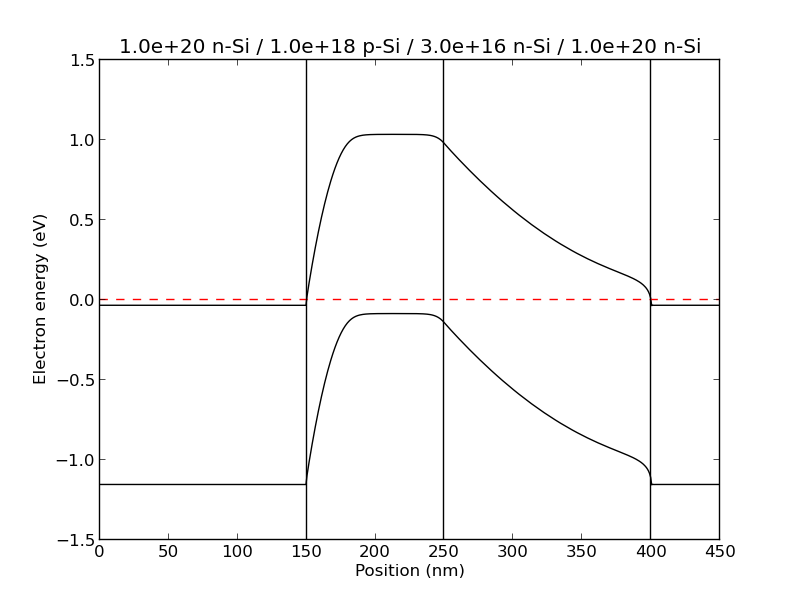
(This one is not expected to be quantitatively accurate, because it involves very heavily doped layers. See below.)
example4(): A depletion region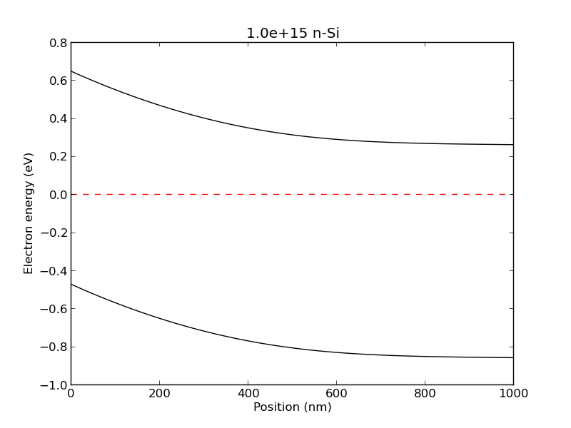
example5(): Comparing to (analytical) depletion approximation for p-n junction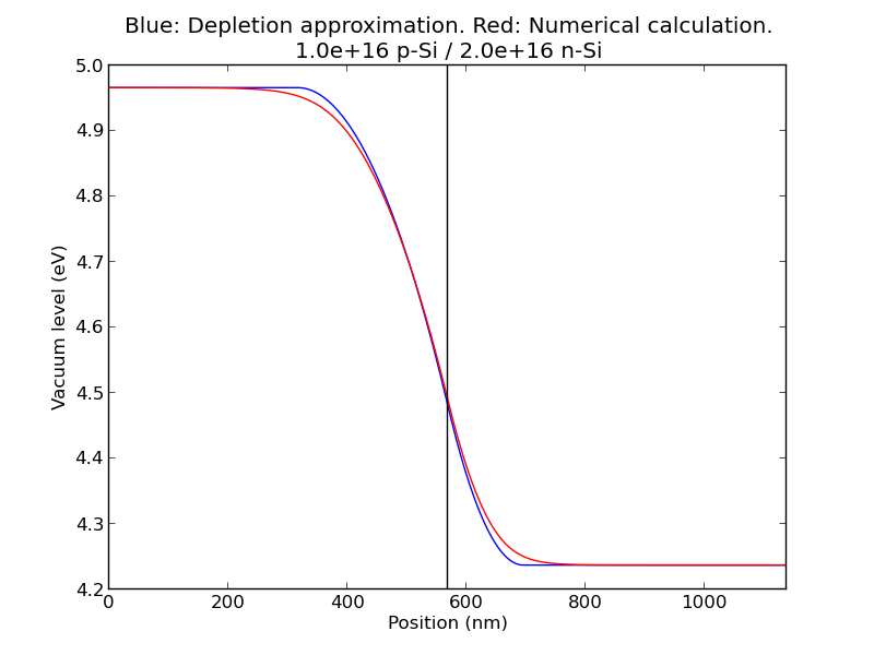
All the code is a single python module. (Written in Python 2.7, but as far as I can tell it should be compatible with Python 3 also. Please email me if you have tried.) It requires numpy and matplotlib. The inner-loop calculation is vectorized in numpy, so the calculation runs quite quickly. (Most plots are generated in ~1 second.) The module requires no setup or compilation, so you can just download it and use it. Or, if you prefer, run
pip install eq_band_diagram
to automatically download it into the default folder.
The functions are all described with docstrings, so if you read the source code you'll hopefully see what's going on. (There is no other documentation besides this page.)
The top of the module contains calc_core(), which has the main algorithm, along with its helper functions local_charge() (which infers charge from vacuum level) and Evac_minus_EF_from_charge() (which infers vacuum level from charge)
The second section of the module contains a more convenient interface / wrapper to the main algorithm. There is a Material class containing density-of-states, electron affinity, and similar such information. (Two Materials are already defined: GaAs and Si.) There is a Layer class that holds a material, thickness, and doping. calc_layer_stack() takes a list of Layers and calls the main algorithm, while plot_bands() displays the result.
The third section of the module contains examples: example1(), ..., example5(). The results are plotted above. This section also has a special function that makes a plot comparing a numerical solution to the depletion approximation, as shown in example5().
The final section of the module has a few test scripts.
Since this is equilibrium, the fermi level is flat. We set it as the zero of energy. Start with the Poisson equation (i.e. Gauss's law):
Evac'' = net_charge / epsilon
(where '' is second derivative in space and Evac is the vacuum energy level.)
(Remember Evac = -electric potential + constant. The minus sign is because Evac is related to electron energy, and electrons have negative charge.) Using finite differences:
(1/2) * dx^2 * Evac''[i] = (Evac[i+1] + Evac[i-1])/2 - Evac[i]
Therefore, the main equation we solve is:
Evac[i] = (Evac[i+1] + Evac[i-1])/2 - (1/2) * dx^2 * net_charge[i] / epsilon
Algorithm: The right-hand-side at the previous time-step gives the left-hand-side at the next time step. A little twist, which suppresses a numerical oscillation, is that net_charge[i] is inferred not from the Evac[i] at the last time step, but instead from the (Evac[i+1] + Evac[i-1])/2 at the last time step.
Boundary values: The boundary values of Evac (i.e., the values at the start of the leftmost layer and the end of the rightmost layer) are kept fixed at predetermined values. You can specify the boundary values yourself, or you can use the default, wherein values are chosen that make the material is charge-neutral at the boundaries.
Seed: Start with the Evac profile wherein everything is charge-neutral, except possibly the first and last points.
Anderson's rule: The vacuum level is assumed to be continuous, so that band alignments are related to electron affinities. Well, that's how the program is written, but you can always lie about the electron affinity in order to get whatever band alignment you prefer.
Nondegenerate electron and hole concentrations: We use formulas like n ~ exp((EF - EC) / kT). So band-filling and nonparabolicity is ignored. This will not be accurate if the electron and hole concentrations are too high.
100% ionized donors and acceptors: It's assumed that all dopants are ionized. Usually that is a pretty safe assumption for common dopants in common semiconductors at higher-than-cryogenic-temperature.
Others: Quantum effects is neglected, etc. etc.