Introduction

Get som arbitrary daily fund data from vanguard and ishares with pandas_datareader (the usual imports are suppressed)

In [1]: start = datetime.datetime(2011, 1, 1)

In [2]: end = datetime.datetime(2016, 1, 1)

In [3]: f = data.DataReader(['VTWG', 'VBK', 'VONG', 'IUSG', 'IUSV',
   ...:                     'VONV', 'VTWV', 'VIOV', 'IJK', 'IVOV'],
   ...:                     'yahoo', start, end)
   ...: 

In [4]: fsp = data.DataReader('^GSPC','yahoo', start, end) # S&P 500

In [5]: fsp = fsp['Adj Close'].pct_change().iloc[1:]

In [6]: rets = f['Adj Close'].pct_change().iloc[1:]

In [7]: rets = rets.apply(lambda x: np.log(1 + x))

In [8]: rets.head(5)
Out[8]: 
                 IJK      IUSG      IUSV      IVOV       VBK      VIOV  \
Date                                                                     
2011-01-04 -0.011640 -0.005500 -0.000811  0.000000 -0.011801 -0.017981   
2011-01-05  0.005343  0.005500  0.005317 -0.003861  0.012180  0.003915   
2011-01-06 -0.002668  0.000211 -0.002771 -0.000336 -0.002020 -0.006042   
2011-01-07 -0.002278 -0.001266 -0.003590 -0.004215 -0.003925 -0.007398   
2011-01-10  0.006623  0.001477 -0.001510  0.002700  0.007457  0.003459   

                VONG      VONV      VTWG      VTWV  
Date                                                
2011-01-04 -0.004230 -0.000525 -0.017888 -0.016540  
2011-01-05  0.005580  0.006113  0.008513  0.007239  
2011-01-06 -0.002363  0.000522 -0.000942 -0.004107  
2011-01-07  0.005057 -0.007687 -0.005989 -0.006109  
2011-01-10 -0.003031 -0.001053  0.010536  0.001655  

Construct a model object with an estimation window of 650 observations and a step size of 12 observations (i.e rebalancing every 12 days)

(these two parameters could be tuned with for ex. cross validation)

In [9]: from entroport import EntroPort

In [10]: ep = EntroPort(rets, 650, 12).fit()

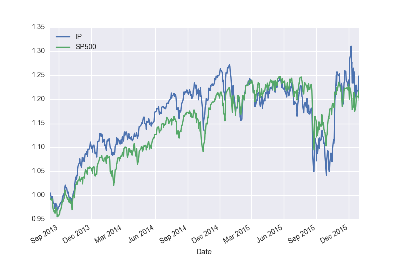
Have a look at the cumulative return

In [11]: (ep.pfs_['ip'] + 1).cumprod().plot();

In [12]: (fsp[ep.pfs_.index[0]:] + 1).cumprod().plot().legend(['IP', 'SP500'], loc=2);

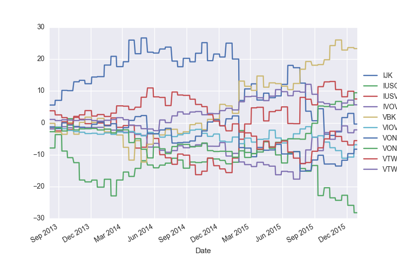
The estimated weights look reasonable (only point estimates are computed) but are noisy¶

In [13]: ep.weights_.plot().legend(loc='center left', bbox_to_anchor=(1, .5));

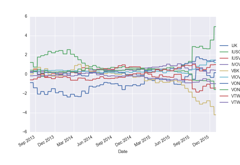
The estimated \(\theta_i\)‘s (the argmin of \(\frac{1}{T} \sum_{t=1}^{T}e^ {\boldsymbol{\theta}' \mathbf{R}_t}\))

In [14]: ep.thetas_.plot().legend(loc='center left', bbox_to_anchor=(1, .5));