ECsPy Reference

This chapter provides a complete reference to all of the functionality included in ECsPy.

Evolutionary Computation

class ecspy.ec.EvolutionExit

An exception that may be raised and caught to end the evolution.

This is an empty exception class that can be raised by the user at any point in the code and caught outside of the evolve method.

class ecspy.ec.Bounder(lower_bound=None, upper_bound=None)

Defines a basic bounding function for numeric lists.

This callable class acts as a function that bounds a numeric list between the lower and upper bounds specified. These bounds can be single values or lists of values. For instance, if the candidate is composed of five values, each of which should be bounded between 0 and 1, you can say Bounder([0, 0, 0, 0, 0], [1, 1, 1, 1, 1]) or just Bounder(0, 1). If either the lower_bound or upper_bound argument is None, the Bounder leaves the candidate unchanged (which is the default behavior).

A bounding function is necessary to ensure that all evolutionary operators respect the legal bounds for candidates. If the user is using only custom operators (which would be aware of the problem constraints), then those can obviously be tailored to enforce the bounds on the candidates themselves. But the built-in operators make only minimal assumptions about the candidate solutions. Therefore, they must rely on an external bounding function that can be user-specified (so as to contain problem-specific information). As a historical note, ECsPy was originally designed to require the maximum and minimum values for all components of the candidate solution to be passed to the evolve method. However, this was replaced by the bounding function approach because it made fewer assumptions about the structure of a candidate (e.g., that candidates were going to be lists) and because it allowed the user the flexibility to provide more elaborate boundings if needed.

In general, a user-specified bounding function must accept two arguments: the candidate to be bounded and the keyword argument dictionary. Typically, the signature of such a function would be bounding_function(candidate, args). This function should return the resulting candidate after bounding has been performed.

Public Attributes:

• lower_bound – the lower bound for a candidate
• upper_bound – the upper bound for a candidate

class ecspy.ec.Individual(candidate=None, maximize=True)

Represents an individual in an evolutionary computation.

An individual is defined by its candidate solution and the fitness (or value) of that candidate solution.

Public Attributes:

• candidate – the candidate solution
• fitness – the value of the candidate solution
• birthdate – the system time at which the individual was created
• maximize – Boolean value stating use of maximization

class ecspy.ec.EvolutionaryComputation(random)

Represents a basic evolutionary computation.

This class encapsulates the components of a generic evolutionary computation. These components are the selection mechanism, the variation operators, the replacement mechanism, the migration scheme, and the observers.

Public Attributes:

• selector – the selection operator
• variator – the (possibly list of) variation operator(s)
• replacer – the replacement operator
• migrator – the migration operator
• archiver – the archival operator
• observer – the (possibly list of) observer(s)
• terminator – the (possibly list of) terminator(s)

The following public attributes do not have legitimate values until after the evolve method executes:

• termination_cause – the name of the function causing evolve to terminate
• generator – the generator function passed to evolve
• evaluator – the evaluator function passed to evolve
• bounder – the bounding function passed to evolve
• maximize – Boolean stating use of maximization passed to evolve
• archive – the archive of individuals
• population – the population of individuals
• num_evaluations – the number of fitness evaluations used
• num_generations – the number of generations processed
• logger – the logger to use (defaults to the logger ‘ecspy.ec’)

Note that the attributes above are, in general, not intended to be modified by the user. (They are intended for the user to query during or after the evolve method’s execution.) However, there may be instances where it is necessary to modify them within other functions. This is possible but should be the exception, rather than the rule.

If logging is desired, the following basic code segment can be used in the main or calling scope to accomplish that:

logger = logging.getLogger('ecspy.ec')
logger.setLevel(logging.DEBUG)
file_handler = logging.FileHandler('ec.log', mode='w')
file_handler.setLevel(logging.DEBUG)
formatter = logging.Formatter('%(asctime)s - %(name)s - %(levelname)s - %(message)s')
file_handler.setFormatter(formatter)
logger.addHandler(file_handler)

Protected Attributes:

• _random – the random number generator object
• _kwargs – the dictionary of keyword arguments initialized from the args parameter in the evolve method

Public Methods:

• evolve – performs the evolution and returns the final archive of individuals

evolve(generator, evaluator, pop_size=100, seeds=[], maximize=True, bounder=<ecspy.ec.Bounder object at 0xa48c9ac>, **args)

Perform the evolution.

This function creates a population and then runs it through a series of evolutionary epochs until the terminator is satisfied. The general outline of an epoch is selection, variation, evaluation, replacement, migration, archival, and observation. The function returns a list of elements of type Individual representing the individuals contained in the final population.

Arguments:

• generator – the function to be used to generate candidate solutions
• evaluator – the function to be used to evaluate candidate solutions
• pop_size – the number of Individuals in the population (default 100)
• seeds – an iterable collection of candidate solutions to include in the initial population (default [])
• maximize – Boolean value stating use of maximization (default True)
• bounder – a function used to bound candidate solutions (default Bounder())
• args – a dictionary of keyword arguments

Note that the _kwargs class variable will be initialized to the args parameter here. It will also be modified to include the following ‘built-in’ keyword arguments:

• _ec – the evolutionary computation (this object)

class ecspy.ec.DEA(random)

Evolutionary computation representing a differential evolutionary algorithm.

This class represents a differential evolutionary algorithm which uses, by default, tournament selection, differential crossover, Gaussian mutation, and steady-state replacement. It is expected that the candidate solution is an iterable object of real values.

Optional keyword arguments in evolve args parameter:

• num_selected – the number of individuals to be selected (default 1)
• tourn_size – the tournament size (default 2)
• crossover_rate – the rate at which crossover is performed (default 1.0)
• differential_phi – the amount of random change in the crossover (default 0.1)
• mutation_rate – the rate at which mutation is performed (default 0.1)
• mean – the mean used in the Gaussian function (default 0)
• stdev – the standard deviation used in the Gaussian function (default 1.0)

class ecspy.ec.EDA(random)

Evolutionary computation representing a canonical estimation of distribution algorithm.

This class represents an estimation of distribution algorithm which uses, by default, truncation selection, estimation of distribution variation, and generational replacement. It is assumed that the candidate solution is an iterable object of real values.

Optional keyword arguments in evolve args parameter:

• num_selected – the number of individuals to be selected (default len(population))
• num_offspring – the number of offspring to create (default 1)
• num_elites – number of elites to consider (default 0)

class ecspy.ec.ES(random)

Evolutionary computation representing a canonical evolution strategy.

This class represents an evolution strategy which uses, by default, the default selection (i.e., all individuals are selected), Gaussian mutation, and ‘plus’ replacement. It is assumed that the candidate solution is an iterable object of real values.

Optional keyword arguments in evolve args parameter:

• mutation_rate – the rate at which mutation is performed (default 0.1)
• mean – the mean used in the Gaussian function (default 0)
• stdev – the standard deviation used in the Gaussian function (default 1.0)
• use_one_fifth_rule – whether the 1/5 rule should be used (default False)

class ecspy.ec.GA(random)

Evolutionary computation representing a canonical genetic algorithm.

This class represents a genetic algorithm which uses, by default, rank selection, n-point crossover, bit-flip mutation, and generational replacement. In the case of bit-flip mutation, it is expected that the candidate solution is an iterable object of binary values.

Optional keyword arguments in evolve args parameter:

• num_selected – the number of individuals to be selected (default 1)
• crossover_rate – the rate at which crossover is performed (default 1.0)
• num_crossover_points – the n crossover points used (default 1)
• mutation_rate – the rate at which mutation is performed (default 0.1)
• num_elites – number of elites to consider (default 0)

class ecspy.ec.SA(random)

Evolutionary computation representing simulated annealing.

Functions

An evolutionary computation is composed of many parts:

• an archiver – stores solutions separate from the population (e.g., in a multiobjective EC)
• an evaluator – measures the fitness of candidate solutions; problem-dependent
• a generator – creates new candidate solutions; problem-dependent
• a migrator – moves individuals to other populations (in the case of distributed ECs)
• observers – view the progress of an EC in operation; may be a list of observers
• a replacer – determines the survivors of a generation
• a selector – determines the parents of a generation
• terminators – determine whether the evolution should stop; may be a list of terminators
• variators – modify candidate solutions; may be a list of variators

Each of these parts may be specified to create custom ECs to suit particular problems.

Archivers

This module provides pre-defined archivers for evolutionary computations.

All archiver functions have the following arguments:

• random – the random number generator object
• population – the population of individuals
• archive – the current archive of individuals
• args – a dictionary of keyword arguments

Each archiver function returns the updated archive.

ecspy.archivers.adaptive_grid_archiver(random, population, archive, args)

Archive only the best individual(s) using a fixed size grid.

This function archives the best solutions by using a fixed-size grid to determine which existing solutions should be removed in order to make room for new ones. This archiver is designed specifically for use with the Pareto Archived Evolution Strategy (PAES).

Optional keyword arguments in args:

• max_archive_size – the maximum number of individuals in the archive (default len(population))
• num_grid_divisions – the number of grid divisions (default 1)

ecspy.archivers.best_archiver(random, population, archive, args)

Archive only the best individual(s).

This function archives the best solutions and removes inferior ones. If the comparison operators have been overloaded to define Pareto preference (as in the Pareto class), then this archiver will form a Pareto archive.

ecspy.archivers.default_archiver(random, population, archive, args)

Archive the current population.

Evaluators

Evaluator functions are problem-specific. This module provides pre-defined evaluators for evolutionary computations.

All evaluator functions have the following arguments:

• candidates – the candidate solutions
• args – a dictionary of keyword arguments

ecspy.evaluators.evaluator(evaluate)

Return an ecspy evaluator function based on the given function.

This function generator takes a function that evaluates only one candidate. The generator handles the iteration over each candidate to be evaluated.

The given function evaluate must have the following signature:

fitness = evaluate(candidate, args)

This function is most commonly used as a function decorator with the following usage:

@evaluator
def evaluate(candidate, args):
    # Implementation of evaluation

The generated function also contains an attribute named single_evaluation which holds the original evaluation function. In this way, the original single-candidate function can be retrieved if necessary.

ecspy.evaluators.parallel_evaluation_mp(candidates, args)

Evaluate the candidates in parallel using multiprocessing.

This function allows parallel evaluation of candidate solutions. It uses the standard multiprocessing library to accomplish the parallelization. The function assigns the evaluation of each candidate to its own job, all of which are then distributed to the available processing units.

parallel_evaluation_mp is the slightly better choice for SMP/multicore parallelism since it does not require you to specify arguments and modules required for evaluation in a non-standard manner. It is, therefore, trivial to set up.

parallel_evaluation_pp supports both SMP / multicore parallelism, as well as distributed computing, which does require you to set up a network of clients.

Note: arguments for the evaluation function should be able to serialize

Required keyword arguments in args:

mp_evaluator – actual evaluation function to be used (This function should have the same signature as any other ecspy evaluation function.)

Optional keyword arguments in args:

• mp_num_cpus – number of processors that will be used (default is machine cpu count)

ecspy.evaluators.parallel_evaluation_pp(candidates, args)

Evaluate the candidates in parallel using Parallel Python.

This function allows parallel evaluation of candidate solutions. It uses the Parallel Python (pp) library to accomplish the parallelization. This library must already be installed in order to use this function. The function assigns the evaluation of each candidate to its own job, all of which are then distributed to the available processing units.

parallel_evaluation_mp is the slightly better choice for SMP/multicore parallelism since it does not require you to specify arguments and modules required for evaluation in a non-standard manner. It is, therefore, trivial to set up.

parallel_evaluation_pp supports both SMP / multicore parallelism, as well as distributed computing, which does require you to set up a network of clients.

Required keyword arguments in args:

pp_evaluator – actual evaluation function to be used (This function should have the same signature as any other ecspy evaluation function.)

Optional keyword arguments in args:

• pp_dependencies – tuple of functional dependencies of the serial evaluator (default ())
• pp_modules – tuple of modules that must be imported for the functional dependencies (default ())
• pp_servers – tuple of servers (on a cluster) that will be used for parallel processing (default (“*”,))

For more information about these arguments, please consult the documentation for Parallel Python.

Generators

Generator functions are problem-specific. They are used to create the initial set of candidate solutions needed by the evolutionary computation. All generator functions have the following arguments:

• random – the random number generator object
• args – a dictionary of keyword arguments

Migrators

This module provides pre-defined migrators for evolutionary computations.

All migrator functions have the following arguments:

• random – the random number generator object
• population – the population of Individuals
• args – a dictionary of keyword arguments

Each migrator function returns the updated population.

class ecspy.migrators.MultiprocessingMigrator(max_migrants=1)

Migrate among processes on the same machine.

This callable class allows individuals to migrate from one process to another on the same machine. It maintains a queue of migrants whose maximum length can be fixed via the max_migrants parameter in the constructor. If the number of migrants in the queue reaches this value, new migrants are not added until earlier ones are consumed. The unreliability of a multiprocessing environment makes it difficult to provide guarantees. However, migrants are theoretically added and consumed at the same rate, so this value should determine the “freshness” of individuals, where smaller queue sizes provide more recency.

An optional keyword argument in args requires the migrant to be evaluated by the current EC before being inserted into the population. This can be important when different populations use different evaluation functions and you need to be able to compare “apples with apples”.

Optional keyword arguments in args:

• evaluate_migrant – should new migrants be evaluated before adding them to the population (default: False)

class ecspy.migrators.NetworkMigrator(server_address, client_addresses, max_migrants=1)

Defines a migration function across a network.

This callable class acts as a migration function that allows candidate solutions to migrate from one population to another via TCP/IP connections.

The migrator is constructed by specifying the IP address of the server (hosting the population from which individuals emigrate) as an IP-port tuple and the addresses of the clients (hosting the populations to which individuals from the server immigrate) as a list of IP-port tuples. The max_migrants parameter specifies the size of the queue of migrants waiting to immigrate to the server from the clients; the newest migrants replace older ones in the queue.

Note: In order to use this migration operator, individuals must be pickle-able.

The following is an example of the use of this operator:

m = NetworkMigrator(('192.168.1.10', 25125),
                    [('192.168.1.11', 12345), ('192.168.1.12', 54321)], 
                    max_migrants=3)

Since the NetworkMigrator object is a server, it should always call the shutdown() method when it is no longer needed, in order to give back its resources.

Public Attributes:

• client_addresses – the list of IP address tuples (IP, port) to which individuals should migrate
• migrants – the deque of migrants (of maximum size specified by max_migrants) waiting to immigrate to client populations

ecspy.migrators.default_migration(random, population, args)

Do nothing.

This function just returns the existing population with no changes.

Observers

This module provides pre-defined observers for evolutionary computations.

All observer functions have the following arguments:

• population – the population of Individuals
• num_generations – the number of elapsed generations
• num_evaluations – the number of candidate solution evaluations
• args – a dictionary of keyword arguments

ecspy.observers.archive_observer(population, num_generations, num_evaluations, args)

Print the current archive to the screen.

ecspy.observers.default_observer(population, num_generations, num_evaluations, args)

Do nothing.

ecspy.observers.file_observer(population, num_generations, num_evaluations, args)

Print the output of the EC to a file.

This function saves the results of the evolutionary computation to two files. The first file, which by default is named ‘ecspy-statistics-file-<timestamp>.csv’, contains the basic generational statistics of the population throughout the run (worst, best, median, and average fitness and standard deviation of the fitness values). The second file, which by default is named ‘ecspy-individuals-file-<timestamp>.csv’, contains every individual during each generation of the run. Both files may be passed to the function as keyword arguments (see below).

Optional keyword arguments in args:

• statistics_file – a file object (default: see text)
• individuals_file – a file object (default: see text)

ecspy.observers.plot_observer(population, num_generations, num_evaluations, args)

Plot the output of the EC as a graph.

This function plots the performance of the EC as a line graph using the pylab library (matplotlib). The graph consists of a blue line representing the best fitness, a green line representing the average fitness, and a red line representing the median fitness. It modifies the keyword arguments variable ‘args’ by including an entry called ‘plot_data’.

If this observer is used, the calling script should also import the pylab library and should end the script with

pylab.show()

Otherwise, the program may generate a runtime error.

ecspy.observers.screen_observer(population, num_generations, num_evaluations, args)

Print the output of the EC to the screen.

This function displays the results of the evolutionary computation to the screen. The output includes the generation number, the current number of evaluations, the average fitness, the maximum fitness, and the full population.

Replacers

This module provides pre-defined replacers for evolutionary computations.

All replacer functions have the following arguments:

• random – the random number generator object
• population – the population of individuals
• parents – the list of parent individuals
• offspring – the list of offspring individuals
• args – a dictionary of keyword arguments

Each replacer function returns the list of surviving individuals.

ecspy.replacers.comma_replacement(random, population, parents, offspring, args)

Performs ‘comma’ replacement.

This function performs ‘comma’ replacement, which means that the entire existing population is replaced by the best population-many elements from the offspring. This function makes the assumption that the size of the offspring is at least as large as the original population. Otherwise, the population size will not be constant.

Optional keyword arguments in args:

use_one_fifth_rule – whether the 1/5 rule should be used (default False)

ecspy.replacers.crowding_replacement(random, population, parents, offspring, args)

Performs crowding replacement as a form of niching.

This function performs crowding replacement, which means that the members of the population are replaced one-at-a-time with each of the offspring. A random sample of crowding_distance individuals is pulled from the current population, and the closest individual to the current offspring (where “closest” is determined by the distance_function) is replaced by that offspring. It is possible for one offspring to replace an earlier offspring in the same generation, given the random sample that is taken of the current survivors for each offspring.

Optional keyword arguments in args:

• distance_function – a function that accepts two candidate solutions and returns the distance between them (default Euclidean L2 distance)
• crowding_distance – a positive integer representing the number of closest solutions to consider as a “crowd” (default 2)

ecspy.replacers.default_replacement(random, population, parents, offspring, args)

Replaces entire population with offspring.

ecspy.replacers.generational_replacement(random, population, parents, offspring, args)

Performs generational replacement with optional weak elitism.

This function performs generational replacement, which means that the entire existing population is replaced by the offspring, truncating to the population size if the number of offspring is larger. Weak elitism may also be specified through the num_elites keyword argument in args. If this is used, the best num_elites individuals in the current population are allowed to survive if they are better than the worst num_elites offspring.

Optional keyword arguments in args:

num_elites – number of elites to consider (default 0)

ecspy.replacers.nsga_replacement(random, population, parents, offspring, args)

Replaces population using the non-dominated sorting technique from NSGA-II.

ecspy.replacers.paes_replacement(random, population, parents, offspring, args)

Replaces population using the Pareto Archived Evolution Strategy method.

ecspy.replacers.plus_replacement(random, population, parents, offspring, args)

Performs ‘plus’ replacement with optional adaptive mutation.

This function performs ‘plus’ replacement, which means that the entire existing population is replaced by the best population-many elements from the combined set of parents and offspring. Adaptive mutation can also be specified here through the use_one_fifth_rule keyword argument in args. This adaptive mutation attempts to keep the rate of viable offspring near 20%. If the number of successful offspring is below 20%, the mutation rate is reduced by 20% (to allow more exploitation). If the number of successful offspring is above 20%, the mutation rate is increased by 20% (to allow more exploration).

Optional keyword arguments in args:

use_one_fifth_rule – whether the 1/5 rule should be used (default False)

ecspy.replacers.random_replacement(random, population, parents, offspring, args)

Performs random replacement with optional weak elitism.

This function performs random replacement, which means that the offspring replace random members of the population, keeping the population size constant. Weak elitism may also be specified through the num_elites keyword argument in args. If this is used, the best num_elites individuals in the current population are allowed to survive if they are better than the worst num_elites offspring.

Optional keyword arguments in args:

num_elites – number of elites to consider (default 0)

ecspy.replacers.simulated_annealing_replacement(random, population, parents, offspring, args)

Replaces population using the simulated annealing schedule.

This function performs simulated annealing replacement based on a temperature and a cooling rate. These can be specified by the keyword arguments ‘temperature’, which should be the initial temperature, and ‘cooling_rate’, which should be the coefficient by which the temperature is reduced. If these keyword arguments are not present, then the function will attempt to base the cooling schedule either on the ratio of evaluations to the maximum allowed evaluations or on the ratio of generations to the maximum allowed generations. Each of these rations is of the form (max - current)/max so that the cooling schedule moves smoothly from 1 to 0.

Optional keyword arguments in args:

• temperature – the initial temperature
• cooling_rate – a real-valued coefficient in the range (0, 1) by which the temperature should be reduced

ecspy.replacers.steady_state_replacement(random, population, parents, offspring, args)

Performs steady-state replacement for the offspring.

This function performs steady-state replacement, which means that the offspring replace the least fit individuals in the existing population, even if those offspring are less fit than the individuals that they replace.

ecspy.replacers.truncation_replacement(random, population, parents, offspring, args)

Replaces population with the best of the population and offspring.

This function performs truncation replacement, which means that the entire existing population is replaced by the best from among the current population and offspring, keeping the existing population size fixed. This is similar to so called ‘plus’ replacement in the evolution strategies literature, except that ‘plus’ replacement considers only parents and offspring for survival. However, if the entire population are parents (which is often the case in ES), then truncation replacement and plus-replacement are equivalent approaches.

Selectors

This module provides pre-defined selectors for evolutionary computations.

All selector functions have the following arguments:

• random – the random number generator object
• population – the population of individuals
• args – a dictionary of keyword arguments

Each selector function returns the list of selected individuals.

ecspy.selectors.default_selection(random, population, args)

Return the population.

This function acts as a default selection scheme for an EC. It simply returns the entire population as having been selected.

ecspy.selectors.fitness_proportionate_selection(random, population, args)

Return fitness proportionate sampling of individuals from the population.

Optional keyword arguments in args:

num_selected – the number of individuals to be selected (default 1)

ecspy.selectors.rank_selection(random, population, args)

Return a rank-based sampling of individuals from the population.

Optional keyword arguments in args:

num_selected – the number of individuals to be selected (default 1)

ecspy.selectors.tournament_selection(random, population, args)

Return a tournament sampling of individuals from the population.

Optional keyword arguments in args:

• num_selected – the number of individuals to be selected (default 1)
• tourn_size – the tournament size (default 2)

ecspy.selectors.truncation_selection(random, population, args)

Selects the best individuals from the population.

This function performs truncation selection, which means that only the best individuals from the current population are selected. This is a completely deterministic selection mechanism.

Optional keyword arguments in args:

num_selected – the number of individuals to be selected (default len(population))

ecspy.selectors.uniform_selection(random, population, args)

Return a uniform sampling of individuals from the population.

This function performs uniform selection by randomly choosing members of the population with replacement.

Optional keyword arguments in args:

num_selected – the number of individuals to be selected (default 1)

Teminators

This module provides pre-defined terminators for evolutionary computations.

All terminator functions have the following arguments:

• population – the population of Individuals
• num_generations – the number of elapsed generations
• num_evaluations – the number of candidate solution evaluations
• args – a dictionary of keyword arguments

ecspy.terminators.average_fitness_termination(population, num_generations, num_evaluations, args)

Return True if the population’s average fitness is near its best fitness.

This function calculates the average fitness of the population, as well as the best fitness. If the difference between those values is less than a specified tolerance, the function returns True.

Optional keyword arguments in args:

tolerance – the minimum allowable difference between average and best fitness (default 0.001)

ecspy.terminators.default_termination(population, num_generations, num_evaluations, args)

Return True.

This function acts as a default termination criterion for an EC.

ecspy.terminators.diversity_termination(population, num_generations, num_evaluations, args)

Return True if population diversity is less than a minimum diversity.

This function calculates the Euclidean distance between every pair of individuals in the population. It then compares the maximum of those distances with a specified minimum required diversity. This terminator is really only well-defined for candidate solutions which are List types of numeric values.

Optional keyword arguments in args:

min_diversity – the minimum population diversity allowed (default 0.001)

ecspy.terminators.evaluation_termination(population, num_generations, num_evaluations, args)

Return True if the number of function evaluations meets or exceeds a maximum.

This function compares the number of function evaluations that have been generated with a specified maximum. It returns True if the maximum is met or exceeded.

Optional keyword arguments in args:

max_evaluations – the maximum candidate solution evaluations (default len(population))

ecspy.terminators.generation_termination(population, num_generations, num_evaluations, args)

Return True if the number of generations meets or exceeds a maximum.

This function compares the number of generations with a specified maximum. It returns True if the maximum is met or exceeded.

Optional keyword arguments in args:

max_generations – the maximum generations (default 1)

ecspy.terminators.time_termination(population, num_generations, num_evaluations, args)

Return True if the elapsed time meets or exceeds a duration of time.

This function compares the elapsed time with a specified maximum. It returns True if the maximum is met or exceeded. If the start_time keyword argument is omitted, it defaults to None and will be set to the current system time (in seconds). If the max_time keyword argument is omitted, it will default to None and will immediately terminate. The max_time argument can be specified in seconds as a floating-point number, as minutes/seconds as a two-element tuple of floating-point numbers, or as hours/minutes/seconds as a three-element tuple of floating-point numbers.

Optional keyword arguments in args:

start_time – the time from which to start measuring (default None) max_time – the maximum time that should elapse (default None)

ecspy.terminators.user_termination(population, num_generations, num_evaluations, args)

Return True if user presses the ESC key when prompted.

This function prompts the user to press the ESC key to terminate the evolution. The prompt persists for a specified number of seconds before evolution continues. Additionally, the function can be customized to allow any press of the ESC key to be stored until the next time this function is called. This function makes use of the msvcrt (Windows) and curses (Unix) libraries. Other operating systems may not be supported.

Optional keyword arguments in args:

• termination_response_timeout – the number of seconds to wait for the user to press the ESC key (default 5)
• clear_termination_buffer – whether the keyboard buffer should be cleared before allowing the user to press a key (default True)

Variators

This module provides pre-defined variators for evolutionary computations.

All variator functions have the following arguments:

• random – the random number generator object
• candidates – the candidate solutions
• args – a dictionary of keyword arguments

Each variator function returns the list of modified individuals.

These variators may make some limited assumptions about the type of candidate solutions on which they operate. These assumptions are noted in the table below.

Variator	Iterable	Indexable	Sliceable	Listable	Lenable	Real	Binary
blend_crossover	X				X	X
differential_crossover	X					X
n_point_crossover			X	X	X
simulated_binary_crossover	X					X
uniform_crossover	X
bit_flip_mutation	X	X			X		X
gaussian_mutation	X	X			X	X
default_variation
estimation_of_distribution_variation		X			X	X

ecspy.variators.crossover(cross)

Return an ecspy crossover function based on the given function.

This function generator takes a function that operates on only two parent candidates to produce an iterable list of offspring (typically two). The generator handles the pairing of selected parents and collecting of all offspring.

The generated function chooses every odd candidate as a ‘mom’ and every even as a ‘dad’ (discounting the last candidate if there is and odd number). For each mom-dad pair, offspring are produced via the cross function.

The given function cross must have the following signature:

offspring = cross(random, mom, dad, args)

This function is most commonly used as a function decorator with the following usage:

@crossover
def cross(random, mom, dad, args):
    # Implementation of paired crossing

The generated function also contains an attribute named single_crossover which holds the original crossover function. In this way, the original single-candidate function can be retrieved if necessary.

ecspy.variators.blend_crossover(random, candidates, args)

Return the offspring of blend crossover on the candidates.

This function assumes that the candidate solutions are iterable and composed of values on which arithmetic operations are defined. It performs blend crossover, which is similar to a generalized averaging of the candidate elements. This function also makes use of the bounder function as specified in the EC’s evolve method.

Optional keyword arguments in args:

• crossover_rate – the rate at which crossover is performed (default 1.0)
• blx_alpha – the blending rate (default 0.1)

ecspy.variators.differential_crossover(random, candidates, args)

Return the offspring of differential crossover on the candidates.

This function assumes that the candidate solutions are iterable and composed of values on which arithmetic operations are defined. It performs differential crossover, which is similar to the update rule used in particle swarm optimization. This function also makes use of the bounder function as specified in the EC’s evolve method.

Optional keyword arguments in args:

• crossover_rate – the rate at which crossover is performed (default 1.0)
• differential_phi – the amount of random change in the crossover (default 0.1)

ecspy.variators.n_point_crossover(random, candidates, args)

Return the offspring of n-point crossover on the candidates.

This function assumes that the candidate solutions are sliceable. It selects n random points without replacement at which to ‘cut’ the candidate solutions and recombine them.

Optional keyword arguments in args:

• crossover_rate – the rate at which crossover is performed (default 1.0)
• num_crossover_points – the n crossover points used (default 1)

ecspy.variators.simulated_binary_crossover(random, candidates, args)

Return the offspring of simulated binary crossover on the candidates.

This function performs simulated binary crosssover, following the implementation in NSGA-II (Deb et al., ICANNGA 1999).

Optional keyword arguments in args:

• sbx_etac – the non-negative distribution index (default 10)

A small value of the sbx_etac optional argument allows solutions far away from parents to be created as children solutions, while a large value restricts only near-parent solutions to be created as children solutions.

ecspy.variators.uniform_crossover(random, candidates, args)

Return the offspring of uniform crossover on the candidates.

This function assumes that the candidate solutions are iterable. For each element of the parents, a biased coin is flipped to determine whether the first offspring gets the ‘mom’ or the ‘dad’ element. An optional keyword argument in args, pux_bias, determines the bias.

Optional keyword arguments in args:

• crossover_rate – the rate at which crossover is performed (default 1.0)
• pux_bias – the bias toward the first candidate in the crossover (default 0.5)

ecspy.variators.mutator(mutate)

Return an ecspy mutator function based on the given function.

This function generator takes a function that operates on only one candidate to produce a mutated candidate. The generator handles the iteration over each candidate in the set of offspring.

The given function mutate must have the following signature:

mutant = mutate(random, candidate, args)

This function is most commonly used as a function decorator with the following usage:

@mutator
def mutate(random, candidate, args):
    # Implementation of mutation

The generated function also contains an attribute named single_mutation which holds the original mutation function. In this way, the original single-candidate function can be retrieved if necessary.

ecspy.variators.bit_flip_mutation(random, candidates, args)

Return the mutants produced by bit-flip mutation on the candidates.

This function assumes that the candidate solution is made of binary values. It performs bit-flip mutation. If a candidate solution contains non-binary values, this function leaves it unchanged.

Optional keyword arguments in args:

mutation_rate – the rate at which mutation is performed (default 0.1)

The mutation rate is applied on a bit by bit basis.

ecspy.variators.gaussian_mutation(random, candidates, args)

Return the mutants created by Gaussian mutation on the candidates.

This function assumes that the candidate solutions are indexable and numeric. It performs Gaussian mutation. This function also makes use of the bounder function as specified in the EC’s evolve method.

Optional keyword arguments in args:

• mutation_rate – the rate at which mutation is performed (default 0.1)
• mean – the mean used in the Gaussian function (default 0)
• stdev – the standard deviation used in the Gaussian function (default 1.0)

ecspy.variators.default_variation(random, candidates, args)

Return the set of candidates without variation.

ecspy.variators.estimation_of_distribution_variation(random, candidates, args)

Return the offspring produced using estimation of distribution.

This function assumes that the candidate solutions are iterable objects containing real values. It creates a statistical model based on the set of candidates. The offspring are then generated from this model. This function also makes use of the bounder function as specified in the EC’s evolve method.

Optional keyword arguments in args:

• num_offspring – the number of offspring to create (default 1)

Particle Swarm Optimization

This module provides capabilities for creating swarm intelligence algorithms.

class ecspy.swarm.PSO(random)

Represents a basic particle swarm optimization algorithm.

This class is built upon the EvolutionaryComputation class making use of an external archive and maintaining the population at the previous timestep, rather than a velocity. This approach was outlined in (Deb and Padhye, “Development of Efficient Particle Swarm Optimizers by Using Concepts from Evolutionary Algorithms”, GECCO 2010, pp. 55–62).

Public Attributes:

• topology – the neighborhood topology (default topologies.star_topology)

Optional keyword arguments in evolve args parameter:

• inertia – the inertia constant to be used in the particle updating
• cognitive_rate – the rate at which the particle’s current position influences its movement (default 2.1)
• social_rate – the rate at which the particle’s neighbors influence its movement (default 2.1)

Topologies

Additionally, particle swarms make use of topologies, which determine the logical relationships among particles in the swarm (i.e., which ones belong to the same “neighborhood”).

This module provides pre-defined topologies for particle swarms.

All topology functions have the following arguments:

• random – the random number generator object
• population – the population of Particles
• args – a dictionary of keyword arguments

Each topology function returns a list of lists of neighbors for each particle in the population. For example, if a swarm contained 10 particles, then this function would return a list containing 10 lists, each of which contained the neighbors for its corresponding particle in the population.

ecspy.topologies.ring_topology(random, population, args)

Returns the neighbors using a ring topology.

This function sets all particles in a specified sized neighborhood as neighbors for a given particle. This is known as a ring topology. The resulting list of lists of neighbors is returned.

Optional keyword arguments in args:

neighborhood_size – the width of the neighborhood around a particle which determines the size of the neighborhood (default 3)

ecspy.topologies.star_topology(random, population, args)

Returns the neighbors using a star topology.

This function sets all particles as neighbors for all other particles. This is known as a star topology. The resulting list of lists of neighbors is returned.

Evolutionary Multiobjective Optimization

This module provides the framework for making multiobjective evolutionary computations.

class ecspy.emo.NSGA2(random)

Evolutionary computation representing the nondominated sorting genetic algorithm.

This class represents the nondominated sorting genetic algorithm (NSGA-II) of Kalyanmoy Deb et al. It uses nondominated sorting with crowding for replacement, binary tournament selection to produce population size children, and a Pareto archival strategy. The remaining operators take on the typical default values but they may be specified by the designer.

class ecspy.emo.PAES(random)

Evolutionary computation representing the Pareto Archived Evolution Strategy.

This class represents the Pareto Archived Evolution Strategy of Joshua Knowles and David Corne. It is essentially a (1+1)-ES with an adaptive grid archive that is used as a part of the replacement process.

class ecspy.emo.Pareto(values=[], maximize=True)

Represents a Pareto multiobjective solution.

A Pareto solution is a multiobjective value that can be compared to other Pareto values using Pareto preference. This means that a solution dominates, or is better than, another solution if it is better than or equal to the other solution in all objectives and strictly better in at least one objective.

Since some problems may mix maximization and minimization among different objectives, an optional maximize parameter may be passed upon construction of the Pareto object. This parameter may be a list of Booleans of the same length as the set of objective values. If this parameter is used, then the maximize parameter of the evolutionary computation’s evolve method should be left as the default True value in order to avoid confusion. (Setting the evolve‘s parameter to False would essentially invert all of the Booleans in the Pareto maximize list.) So, if all objectives are of the same type (either maximization or minimization), then it is best simply to use the maximize parameter of the evolve method and to leave the maximize parameter of the Pareto initialization set to its default True value. However, if the objectives are mixed maximization and minimization, it is best to leave the evolve‘s maximize parameter set to its default True value and specify the Pareto’s maximize list to the appropriate Booleans.

Analysis

This module provides analysis methods for the results of evolutionary computations.

ecspy.analysis.generation_plot(filename, errorbars=True)

Plot the results of the EC using generation statistics.

This function creates a plot of the generation fitness statistics (best, worst, median, and average).

An example image saved from the generation_plot function (without error bars).

Arguments:

• filename – the name of the statistics file produced by the file_observer
• errorbars – Boolean value stating whether standard error bars should be drawn (default True)

ecspy.analysis.hypervolume(pareto_set, reference_point=None)

Calculates the hypervolume by slicing objectives (HSO).

This function calculates the hypervolume (or S-measure) of a nondominated set using the Hypervolume by Slicing Objectives (HSO) procedure of While, et al. (IEEE CEC 2005). The pareto_set should be a list of lists of objective values. The reference_point may be specified or it may be left as the default value of None. In that case, the reference point is calculated to be the maximum value in the set for all objectives (the ideal point). This function assumes that objectives are to be maximized.

Arguments:

• pareto_set – the list or lists of objective values comprising the Pareto front
• reference_point – the reference point to be used (default None)

Benchmark Problems

class ecspy.benchmarks.Benchmark(dimensions, objectives=1)

Defines a global optimization benchmark problem.

This abstract class defines the basic structure of a global optimization problem. Subclasses should implement the generator and evaluator methods for a particular optimization problem, which can be used with ECsPy evolutionary computations.

In addition to being used with evolutionary computations, subclasses of this are also callable. the arguments passed to such a call are combined into a list and passed as the single candidate to the evaluator method. The single calculated fitness is returned.

Public Attributes:

• dimensions – the number of inputs to the problem
• objectives – the number of outputs of the problem (default 1)
• bounder – the bounding function for the problem (default None)
• maximize – whether the problem is one of maximization (default True)

class ecspy.benchmarks.Binary(benchmark, dimension_bits)

Defines a binary problem based on an existing benchmark problem.

This class can be used to modify an existing benchmark problem to allow it to use a binary representation. The generator creates a list of binary values of size dimensions x dimension_bits. The evaluator accepts a candidate represented by such a binary list and transforms that candidate into a real-valued list as follows:

1. Each set of dimension_bits bits is converted to its positive integer representation.
2. Next, that integer value is divided by the maximum integer that can be represented by dimension_bits bits to produce a real number in the range [0, 1].
3. That real number is then scaled to the range [lower_bound, upper_bound] for that dimension (which should be defined by the bounder).

Public Attributes:

• benchmark – the original benchmark problem
• dimension_bits – the number of bits to use to represent each dimension
• bounder – the bounding function for the underlying benchmark problem
• maximize – whether the underlying benchmark problem is one of maximization

Single-Objective Benchmarks

class ecspy.benchmarks.Ackley(dimensions=2)

Defines the Ackley benchmark problem.

This class defines the Ackley global optimization problem. This is a multimodal minimization problem defined as follows:

Here, represents the number of dimensions and for .

Two-dimensional Ackley function (image source)

Public Attributes:

• global_optimum – the problem input that produces the optimum output. Here, this corresponds to [0, 0, ..., 0].

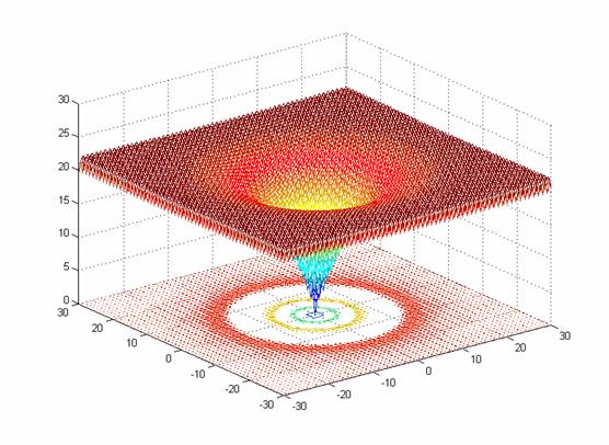
class ecspy.benchmarks.Griewank(dimensions=2)

Defines the Griewank benchmark problem.

This class defines the Griewank global optimization problem. This is a highly multimodal minimization problem with numerous, wide-spread, regularly distributed local minima. It is defined as follows:

Here, represents the number of dimensions and for .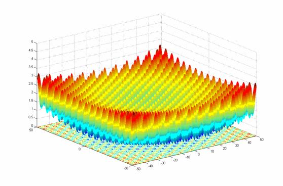

Two-dimensional Griewank function (image source)

Public Attributes:

• global_optimum – the problem input that produces the optimum output. Here, this corresponds to [0, 0, ..., 0].

class ecspy.benchmarks.Rastrigin(dimensions=2)

Defines the Rastrigin benchmark problem.

This class defines the Rastrigin global optimization problem. This is a highly multimodal minimization problem where the local minima are regularly distributed. It is defined as follows:

Here, represents the number of dimensions and for .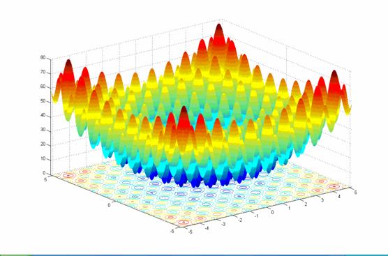

Two-dimensional Rastrigin function (image source)

Public Attributes:

• global_optimum – the problem input that produces the optimum output. Here, this corresponds to [0, 0, ..., 0].

class ecspy.benchmarks.Rosenbrock(dimensions=2)

Defines the Rosenbrock benchmark problem.

This class defines the Rosenbrock global optimization problem, also known as the “banana function.” The global optimum sits within a narrow, parabolic-shaped flattened valley. It is defined as follows:

Here, represents the number of dimensions and for .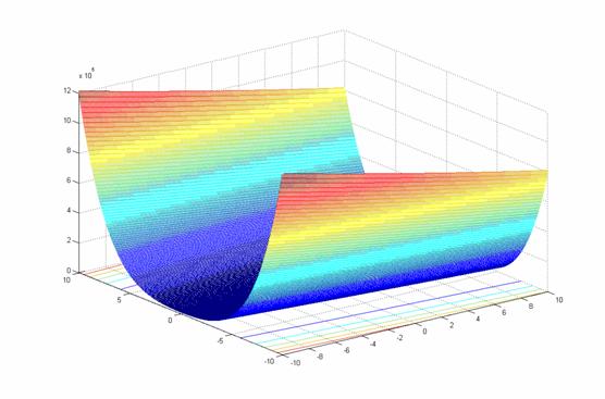

Two-dimensional Rosenbrock function (image source)

Public Attributes:

• global_optimum – the problem input that produces the optimum output. Here, this corresponds to [1, 1, ..., 1].

class ecspy.benchmarks.Schwefel(dimensions=2)

Defines the Schwefel benchmark problem.

This class defines the Schwefel global optimization problem. It is defined as follows:

Here, represents the number of dimensions and for .

Two-dimensional Schwefel function (image source)

Public Attributes:

• global_optimum – the problem input that produces the optimum output. Here, this corresponds to [420.9687, 420.9687, ..., 420.9687].

class ecspy.benchmarks.Sphere(dimensions=2)

Defines the Sphere benchmark problem.

This class defines the Sphere global optimization problem, also called the “first function of De Jong’s” or “De Jong’s F1.” It is continuous, convex, and unimodal, and it is defined as follows:

Here, represents the number of dimensions and for .

Two-dimensional Sphere function (image source)

Public Attributes:

• global_optimum – the problem input that produces the optimum output. Here, this corresponds to [0, 0, ..., 0].

Multi-Objective Benchmarks

class ecspy.benchmarks.Kursawe(dimensions=2)

Defines the Kursawe multiobjective benchmark problem.

This class defines the Kursawe multiobjective minimization problem. This function accepts an n-dimensional input and produces a two-dimensional output. It is defined as follows:

Here, represents the number of dimensions and for .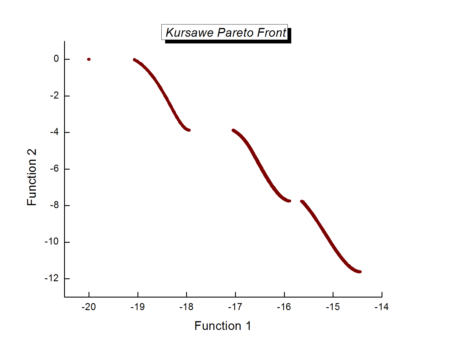

Three-dimensional Kursawe Pareto front (image source)

class ecspy.benchmarks.DTLZ1(dimensions=2, objectives=2)

Defines the DTLZ1 multiobjective benchmark problem.

This class defines the DTLZ1 multiobjective minimization problem. taken from (Deb et al., “Scalable Multi-Objective Optimization Test Problems.” CEC 2002, pp. 825–830). This function accepts an n-dimensional input and produces an m-dimensional output. It is defined as follows:

Here, represents the number of dimensions, represents the number of objectives, for , and

The recommendation given in the paper mentioned above is to provide 4 more dimensions than objectives. For instance, if we want to use 2 objectives, we should use 6 dimensions.

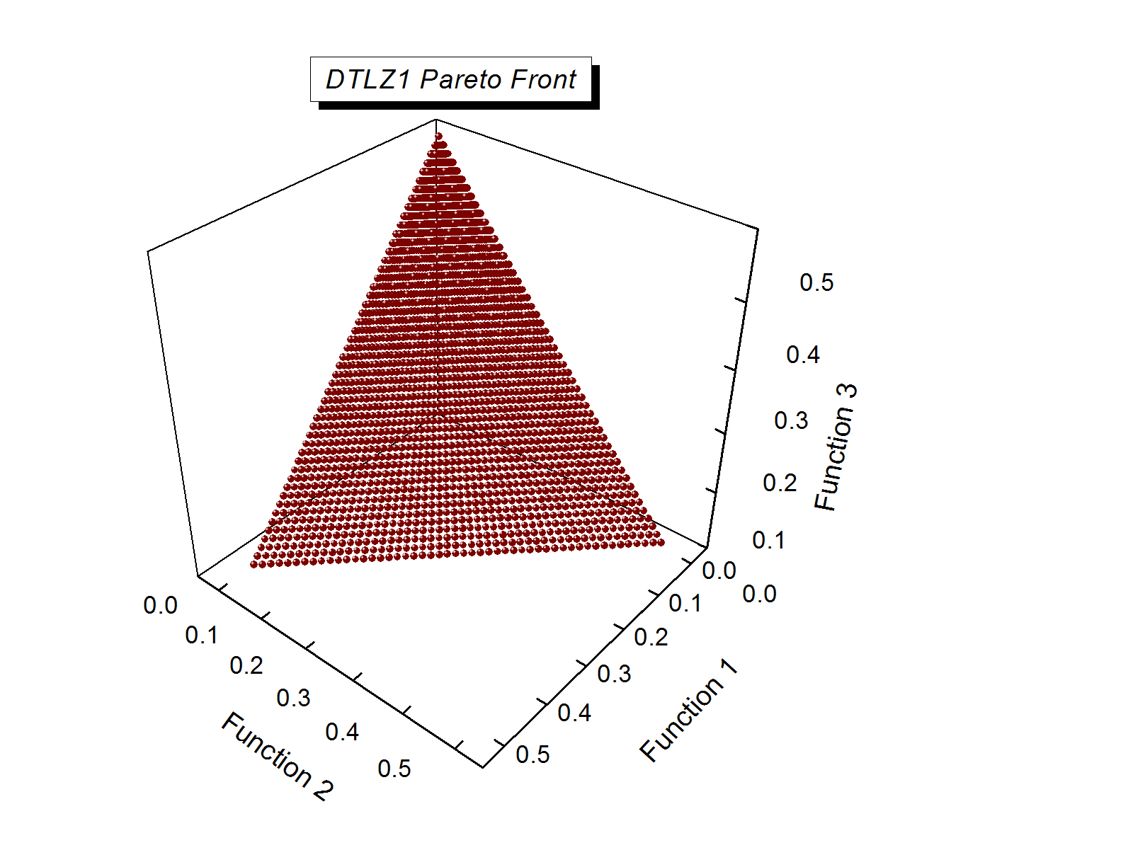
Three-dimensional DTLZ1 Pareto front (image source)

class ecspy.benchmarks.DTLZ2(dimensions=2, objectives=2)

Defines the DTLZ2 multiobjective benchmark problem.

This class defines the DTLZ2 multiobjective minimization problem. taken from (Deb et al., “Scalable Multi-Objective Optimization Test Problems.” CEC 2002, pp. 825–830). This function accepts an n-dimensional input and produces an m-dimensional output. It is defined as follows:

Here, represents the number of dimensions, represents the number of objectives, for , and

The recommendation given in the paper mentioned above is to provide 9 more dimensions than objectives. For instance, if we want to use 2 objectives, we should use 11 dimensions.

class ecspy.benchmarks.DTLZ3(dimensions=2, objectives=2)

Defines the DTLZ3 multiobjective benchmark problem.

This class defines the DTLZ3 multiobjective minimization problem. taken from (Deb et al., “Scalable Multi-Objective Optimization Test Problems.” CEC 2002, pp. 825–830). This function accepts an n-dimensional input and produces an m-dimensional output. It is defined as follows:

Here, represents the number of dimensions, represents the number of objectives, for , and

The recommendation given in the paper mentioned above is to provide 9 more dimensions than objectives. For instance, if we want to use 2 objectives, we should use 11 dimensions.

class ecspy.benchmarks.DTLZ4(dimensions=2, objectives=2, alpha=100)

Defines the DTLZ4 multiobjective benchmark problem.

This class defines the DTLZ4 multiobjective minimization problem. taken from (Deb et al., “Scalable Multi-Objective Optimization Test Problems.” CEC 2002, pp. 825–830). This function accepts an n-dimensional input and produces an m-dimensional output. It is defined as follows:

Here, represents the number of dimensions, represents the number of objectives, for , and

The recommendation given in the paper mentioned above is to provide 9 more dimensions than objectives. For instance, if we want to use 2 objectives, we should use 11 dimensions.

class ecspy.benchmarks.DTLZ5(dimensions=2, objectives=2)

Defines the DTLZ5 multiobjective benchmark problem.

This class defines the DTLZ5 multiobjective minimization problem. taken from (Deb et al., “Scalable Multi-Objective Optimization Test Problems.” CEC 2002, pp. 825–830). This function accepts an n-dimensional input and produces an m-dimensional output. It is defined as follows:

Here, represents the number of dimensions, represents the number of objectives, for , and

The recommendation given in the paper mentioned above is to provide 9 more dimensions than objectives. For instance, if we want to use 2 objectives, we should use 11 dimensions.

class ecspy.benchmarks.DTLZ6(dimensions=2, objectives=2)

Defines the DTLZ6 multiobjective benchmark problem.

This class defines the DTLZ6 multiobjective minimization problem. taken from (Deb et al., “Scalable Multi-Objective Optimization Test Problems.” CEC 2002, pp. 825–830). This function accepts an n-dimensional input and produces an m-dimensional output. It is defined as follows:

Here, represents the number of dimensions, represents the number of objectives, for , and

The recommendation given in the paper mentioned above is to provide 9 more dimensions than objectives. For instance, if we want to use 2 objectives, we should use 11 dimensions.

class ecspy.benchmarks.DTLZ7(dimensions=2, objectives=2)

Defines the DTLZ7 multiobjective benchmark problem.

This class defines the DTLZ7 multiobjective minimization problem. taken from (Deb et al., “Scalable Multi-Objective Optimization Test Problems.” CEC 2002, pp. 825–830). This function accepts an n-dimensional input and produces an m-dimensional output. It is defined as follows:

Here, represents the number of dimensions, represents the number of objectives, for , and

The recommendation given in the paper mentioned above is to provide 19 more dimensions than objectives. For instance, if we want to use 2 objectives, we should use 21 dimensions.

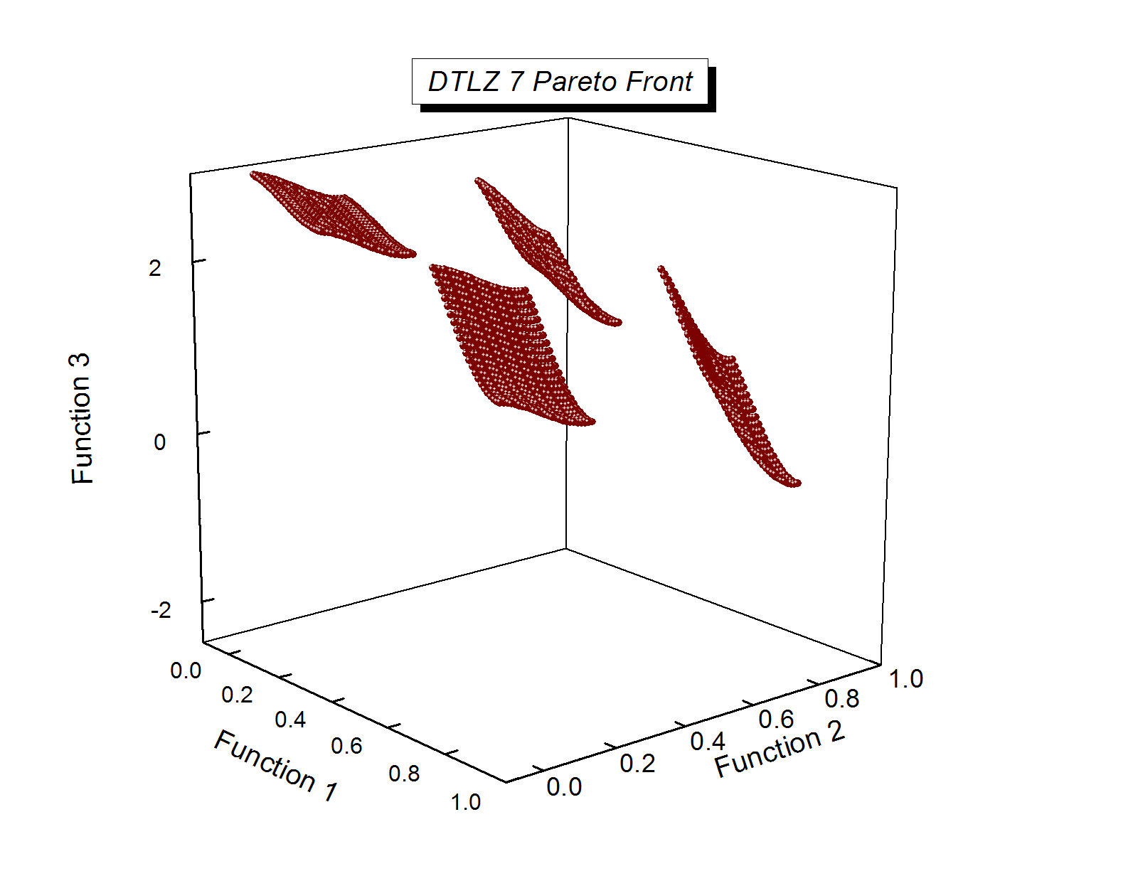
Three-dimensional DTLZ7 Pareto front (image source)

Contributed Utilities

class ecspy.contrib.utils.instantiated(target)

Create a instantiated version of a function.

This function allows an ordinary function passed to it to act very much like a callable instance of a class. For ecspy, this means that evolutionary operators (selectors, variators, replacers, etc.) can be created as normal functions and then be given the ability to have attributes that are specific to the instance. Python functions can always have attributes without employing any special mechanism, but those attributes exist for the function, and there is no way to create a new “instance” except by implementing a new function with the same functionality. This class provides a way to “instantiate” the same function multiple times in order to provide each “instance” with its own set of independent attributes.

The attributes that are created on a instantiated function are passed into that function via the ubiquitous args variable in ecspy. Any user-specified attributes are added to the args dictionary and replace any existing entry if necessary. If the function modifies those entries in the dictionary (e.g., when dynamically modifying parameters), the corresponding attributes are modified as well.

Note that this class makes heavy use of run-time inspection provided by the inspect core library.

The typical usage is as follows:

def typical_function(*args, **kwargs):
    # Implementation of typical function

fun_one = instantiated(typical_function)
fun_two = instantiated(typical_function)
fun_one.attribute = value_one
fun_two.attribute = value_two

class ecspy.contrib.utils.memoized(target)

Cache a function’s return value each time it is called.

This function serves as a function decorator to provide a caching of evaluated fitness values. If called later with the same arguments, the cached value is returned instead of being re-evaluated.

This decorator assumes that candidates can be converted into tuple objects to be used for hashing into a dictionary. It should be used when evaluating an expensive fitness function to avoid costly re-evaluation of those fitnesses. The typical usage is as follows:

@memoized
def expensive_fitness_function(candidates, args):
    # Implementation of expensive fitness calculation